Quantum Tunneling, Part 3

Last time, we solved the problem of a rectangular potential barrier by deriving the tunneling probability of a quantum particle. Today, we will attempt to solve the problem numerically by simulating a particle hitting a potential barrier and, hopefully, tunneling through it.

---

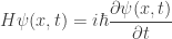
One thing to note: the analytic solution from last time was that of a time-independent problem. However, writing a simulation to model the same case is, frankly, boring. Instead, let us simulate the time dependent problem represented by the Schrödinger equation:

Moreover, instead of having the wave function represent a plane wave solution, we will look at the time evolution of a localized Gaussian wave packet.

We start by importing several packages. In particular, we will require the sparse package to represent sparse matrices, and the sparse.linalg module to manipulate them:

import matplotlib
matplotlib.use('Qt4Agg')
import matplotlib.pyplot as plt 
import scipy as sp
from scipy.sparse import linalg as ln
from scipy import sparse as sparse
import matplotlib.animation as animation

Next, we create the Wave_Packet class. It will require multiple parameters to instantiate:

class Wave_Packet:
    def __init__(self, n_points, dt, sigma0=5.0, k0=1.0, x0=-150.0, x_begin=-200.0,
                 x_end=200.0, barrier_height=1.0, barrier_width=3.0):

        self.n_points = n_points
        self.sigma0 = sigma0
        self.k0 = k0
        self.x0 = x0
        self.dt = dt
        self.prob = sp.zeros(n_points)
        self.barrier_width = barrier_width
        self.barrier_height = barrier_height
        
        """ 1) Space discretization """
        self.x, self.dx = sp.linspace(x_begin, x_end, n_points, retstep=True)        

        """ 2) Initialization of the wave function to Gaussian wave packet """
        norm = (2.0 * sp.pi * sigma0**2)**(-0.25)
        self.psi = sp.exp(-(self.x - x0)**2 / (4.0 * sigma0**2))
        self.psi *= sp.exp(1.0j * k0 * self.x)
        self.psi *= (2.0 * sp.pi * sigma0**2)**(-0.25)

        """ 3) Setting up the potential barrier """
        self.potential = sp.array(
            [barrier_height if 0.0 < x < barrier_width else 0.0 for x in self.x])

        """ 4) Creating the Hamiltonian """
        h_diag = sp.ones(n_points) / self.dx**2 + self.potential
        h_non_diag = sp.ones(n_points - 1) * (-0.5 / self.dx**2)
        hamiltonian = sparse.diags([h_diag, h_non_diag, h_non_diag], [0, 1, -1])
        
        """ 5) Computing the Crank-Nicolson time evolution matrix """
        implicit = (sparse.eye(self.n_points) - dt / 2.0j * hamiltonian).tocsc()
        explicit = (sparse.eye(self.n_points) + dt / 2.0j * hamiltonian).tocsc() 
        self.evolution_matrix = ln.inv(implicit).dot(explicit).tocsr()

We then carry on as follows:

1. Discretize space using a uniformly spaced grid x of step dx.
2. Initialize the wave function as a Gaussian packet. We first prepare a Gaussian distribution of deviation sigma0 centered at x0, which we then multiply by a complex exponential representing the initial momentum k0, and finally normalize:

3. Set up the potential as a zero array, except for the barrier which is located just to the right of the origin of the coordinate system.
4. Calculate the Hamiltonian matrix. Here we adopt the atomic unit system, in which the Hamiltonian assumes the simple form:

The action of the Laplace operator on a generic function can be discretized according to the finite difference scheme:

and hence the Laplace operator itself may be represented by the finite difference stencil . Taking the potential into account as well, the discretized Hamiltonian takes the form of the matrix:

In the script, we first create the arrays representing the diagonal and off-diagonal elements. Then, we use the sparse.diag() function to build a sparse matrix by specifying the diagonal elements and their respective distance from the main diagonal:

class Wave_Packet:
    ...
        """ 4) Creating the Hamiltonian """
        h_diag = sp.ones(n_points) / self.dx**2 + self.potential
        h_non_diag = sp.ones(n_points - 1) * (-0.5 / self.dx**2)
        hamiltonian = sparse.diags([h_diag, h_non_diag, h_non_diag], [0, 1, -1])
    ...

5. Finally, compute the time evolution operator. Given our differential equation:

we can discretize it in time as:

This is called the forward Euler method, or the explicit method, as we can easily express the value of the desired function at the next time step from its value at the current step. Likewise, we can carry out a backward Euler method by imposing:

This, instead, is an implicit formula — the value of the function at the next time step is present on both sides of the equation.

Combining these two methods yields the so-called Crank-Nicolson scheme, which combines adequate accuracy and stability, and incurs a relatively modest computational cost:

Isolating the value of we eventually get:

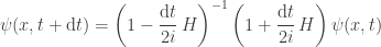
Thus, we create the implicit and explicit matrices. According to the documentation, the matrix to be inverted should be in the compressed sparse column (csc) format for maximum performance, hence we convert both matrices to the csc representation. However, matrix-vector multiplication is faster when the matrix is in the compressed sparse row (csr) format:

class Wave_Packet:
    ...
        """ 5) Computing the Crank-Nicolson time evolution matrix """
        implicit = (sparse.eye(self.n_points) - dt / 2.0j * hamiltonian).tocsc()
        explicit = (sparse.eye(self.n_points) + dt / 2.0j * hamiltonian).tocsc() 
        self.evolution_matrix = ln.inv(implicit).dot(explicit).tocsr()

---

Now that we set everything up nicely, the method evolve(), which takes care of advancing the state of the system one step ahead in time, can be quite simple and straightforward:

class Wave_Packet:
    ...
    def evolve(self):
        self.psi = self.evolution_matrix.dot(self.psi)
        self.prob = abs(self.psi)**2

        norm = sum(self.prob)
        self.prob /= norm
        self.psi /= norm**0.5

        return self.prob

We first compute the wave function at the next time step by applying the time evolution matrix to the previous wave function. What we are interested in, however, is the probability density — modulus square of the wave function. Before we return the density, we normalize both quantities.

Animation

As we have done something very similar in a recent post, we will move quickly here. In the constructor, apart from setting up the figure, we plot the potential barrier (its height reduced, just for a nicer visual presentation), as well as display a timer:

class Animator:
    def __init__(self, wave_packet):
        self.time = 0.0
        self.wave_packet = wave_packet
        self.fig, self.ax = plt.subplots()
        plt.plot(self.wave_packet.x, self.wave_packet.potential * 0.1, color='r')
        
        self.time_text = self.ax.text(0.05, 0.95, '', horizontalalignment='left',
            verticalalignment='top', transform=self.ax.transAxes)
        self.line, = self.ax.plot(self.wave_packet.x, self.wave_packet.evolve())
        self.ax.set_ylim(0, 0.2)
        self.ax.set_xlabel('Position (a$_0$)')
        self.ax.set_ylabel('Probability density (a$_0$)')

    ...

The update(data) method simply updates the plot of the probability density. The actual data to be plotted at each time step is computed in the time_step() method. The return value of the wave_packet is yielded at each call of the method. We also take car of updating the time display. Note that we are working in atomic units in general, but convert to SI here for the sake of clarity. Finally, the animate() method takes care of creating the animation:

class Animator:
    ...
    def update(self, data):
        self.line.set_ydata(data)
        return self.line,
    
    def time_step(self):
        while True:
            self.time += self.wave_packet.dt
            self.time_text.set_text(
                'Elapsed time: {:6.2f} fs'.format(self.time * 2.419e-2))
          
            yield self.wave_packet.evolve()
    
    def animate(self):
        self.ani = animation.FuncAnimation(
            self.fig, self.update, self.time_step, interval=5, blit=False)

Results and Discussion

Let’s set up a quantum particle with a Gaussian profile on a collision course with a potential barrier. What will happen?

Part of the particle appears to tunnel through the barrier! If we were to place a detector behind the barrier, it might measure the particle appearing behind it — although the probability of that will be quite a bit lower compared to the chance of finding the particle in front of the barrier, where we classically expect it to be.

The system behaves as we hoped it would — qualitatively, that is. But does the simulation agree with our predictions quantitatively as well? Let us integrate the probability density on both sides of the barrier at each time step. What we observe is, naturally, that the probability of the particle being on the left of the barrier starts out equal to one, but after a few femtoseconds the particle tunnels through and we have a non-zero probability to observe it on the right of the barrier:

The ratio of the probability to the right and to the left of the barrier gives us the tunneling probability — or transmission coefficient, as we called it last time:

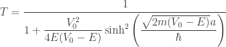
To verify a possible quantitative agreement of our numerical model with the above equation, I’ve run several simulations with different barrier widths and heights:

Tunneling probability as a function of barrier width (top) and height (bottom). The points represent simulation results, the full line corresponds to the analytic solution.

The agreement is not perfect. In all honesty, I had to play around a bit with some of the parameters in the analytic solution to better match the curve to the data points. However, a perfect correlation is not expected — the analytic solution was derived for plane waves, whereas here we simulate a wave packet. In any case, we observe what seems like the correct behaviour: the thicker and higher the barrier, the lower the probability of the particle tunneling through it.

This is the last post in the current series. Until next time!

---

For the sake of convenience, you can find the whole script below:

import matplotlib
matplotlib.use('Qt4Agg')
import matplotlib.pyplot as plt 
import scipy as sp
from scipy.sparse import linalg as ln
from scipy import sparse as sparse
import matplotlib.animation as animation

class Wave_Packet:
    def __init__(self, n_points, dt, sigma0=5.0, k0=1.0, x0=-150.0, x_begin=-200.0,
                 x_end=200.0, barrier_height=1.0, barrier_width=3.0):

        self.n_points = n_points
        self.sigma0 = sigma0
        self.k0 = k0
        self.x0 = x0
        self.dt = dt
        self.prob = sp.zeros(n_points)
        self.barrier_width = barrier_width
        self.barrier_height = barrier_height
        
        """ 1) Space discretization """
        self.x, self.dx = sp.linspace(x_begin, x_end, n_points, retstep=True)        

        """ 2) Initialization of the wave function to Gaussian wave packet """
        norm = (2.0 * sp.pi * sigma0**2)**(-0.25)
        self.psi = sp.exp(-(self.x - x0)**2 / (4.0 * sigma0**2))
        self.psi *= sp.exp(1.0j * k0 * self.x)
        self.psi *= (2.0 * sp.pi * sigma0**2)**(-0.25)

        """ 3) Setting up the potential barrier """
        self.potential = sp.array(
            [barrier_height if 0.0 < x < barrier_width else 0.0 for x in self.x])

        """ 4) Creating the Hamiltonian """
        h_diag = sp.ones(n_points) / self.dx**2 + self.potential
        h_non_diag = sp.ones(n_points - 1) * (-0.5 / self.dx**2)
        hamiltonian = sparse.diags([h_diag, h_non_diag, h_non_diag], [0, 1, -1])
        
        """ 5) Computing the Crank-Nicolson time evolution matrix """
        implicit = (sparse.eye(self.n_points) - dt / 2.0j * hamiltonian).tocsc()
        explicit = (sparse.eye(self.n_points) + dt / 2.0j * hamiltonian).tocsc() 
        self.evolution_matrix = ln.inv(implicit).dot(explicit).tocsr()

    def evolve(self):
        self.psi = self.evolution_matrix.dot(self.psi)
        self.prob = abs(self.psi)**2

        norm = sum(self.prob)
        self.prob /= norm
        self.psi /= norm**0.5

        return self.prob

class Animator:
    def __init__(self, wave_packet):
        self.time = 0.0
        self.wave_packet = wave_packet
        self.fig, self.ax = plt.subplots()
        plt.plot(self.wave_packet.x, self.wave_packet.potential * 0.1, color='r')
        
        self.time_text = self.ax.text(0.05, 0.95, '', horizontalalignment='left',
            verticalalignment='top', transform=self.ax.transAxes)
        self.line, = self.ax.plot(self.wave_packet.x, self.wave_packet.evolve())
        self.ax.set_ylim(0, 0.2)
        self.ax.set_xlabel('Position (a$_0$)')
        self.ax.set_ylabel('Probability density (a$_0$)')

    def update(self, data):
        self.line.set_ydata(data)
        return self.line,
    
    def time_step(self):
        while True:
            self.time += self.wave_packet.dt
            self.time_text.set_text(
                'Elapsed time: {:6.2f} fs'.format(self.time * 2.419e-2))
          
            yield self.wave_packet.evolve()
    
    def animate(self):
        self.ani = animation.FuncAnimation(
            self.fig, self.update, self.time_step, interval=5, blit=False)


wave_packet = WavePacket(n_points=500, dt=0.5, barrier_width=10, barrier_height=1)
animator = Animator(wave_packet)
animator.animate()
plt.show()