Counting Stars (With Python and Pandas)

How many stars are there in the night sky? A hundred? A thousand? Ten thousand? A hundred thousand? We could just go to Wikipedia, but that’d be lame. We could also go out tonight (provided the weather is nice) and try to count. It would be an exercise in patience, and ultimately, in futility. Mad respect to those past astronomers who catalogued the sky with little more than their eyes and a piece of paper. Maybe we could select a small part of sky, count the stars, then extrapolate from there. But no, we won’t do any of that today.

Today, we will look at the results of the Hipparcos survey, one of the first, large scale surveys of our galactic neighborhood. More than 118’000 stars have been observed over extended periods of time, and their brightness and parallax were measured. Follow-up studies have blown this initial survey out of the water, with up to billions (!) of objects in the night sky sampled — but that is too much data to go over here. For now, we will simply obtain, parse, and analyze the data from the more humble Hipparcos project, and try to answer the initial question: how many stars are there in the night sky?

The Hipparcos Survey

Hipparcos, or the High Precision Parallax Collecting Satellite, and also a play on the name of the ancient Greek astronomer Hipparcus, was a mission by the European Space Agency with the goal of mapping the motion, brightness, and parallax of more than a hundred thousand stars. The satellite launched in 1989, and for 4 years analyzed the 118’000-something predefined objects. The majority of the stars to be observed were selected based on their apparent magnitude — practically all stars potentially visible to the naked eye were included in that input list.

It took another 4 years to comb through the observational data, and compile a catalogue of the positions, velocities, as well as distances of the studied stars, in addition to a plethora of photometric data. The catalogue can be accessed here (in a plain text format), with an explanatory document here. As you can easily see, it is a mess.

Wrestling the Data into a DataFrame

Let us first inspect the data file:

The columns are separated by the | character, and most relevant data appears to be in its own column. The exception here is the position of the star, which is given by two values (right ascension, or RAdeg, and declination, or DEdeg, both measured in degrees) in a single column. Not shown in the image above, but also present, are the standard deviations of all astrometric data. Likewise, photometric quantities are included for most stars, however, those won’t be relevant for us now.

We thus import the relevant libraries (pandas, numpy, and pyplot, notably):

import pandas as pd
import numpy as np
from matplotlib import pyplot as plt

And start with reading the input data as a CSV file. We specify the delimiter to be |, skip the first 11 as well as the last row, and tell pandas to ignore the header. Next, we want the parser to only care about specific columns. The list of columns passed to the usecols argument and the list of labels passed to the column names argument should make clear what data we are interested in:

import pandas as pd
import numpy as np
from matplotlib import pyplot as plt
import seaborn as sns

def parse_input_file(filename):
    data = pd.read_csv(filename, delimiter='|', engine='python',
                   skiprows=11, 
                   skipfooter=1,
                   index_col=0,
                   header=0,
                   usecols=[1, 4, 7, 9, 10, 11, 12, 13, 14, 15, 16],
                   names=['index', 'magnitude', 'raw position', 'parallax', 
                          'proper motion alpha', 'proper motion delta',
                          'error alpha', 'error delta', 'error parallax',
                          'error motion alpha', 'error motion delta'])
    
    # convert position string into two floats for the two position coordinates
    data = parse_raw_position(data)
    
    # remove rows with NaN values (data missing)
    data.dropna(inplace=True)
  
    # convert all miliarcsecond values to degrees
    data = convert_to_degrees(data)
    
    # reinterpret magnitude values as floats
    data['magnitude'] = data['magnitude'].astype(float)
    
    return data

Once the data is read in, we need to take care of a few issues. First, the position of each star is determined by two numbers present in the same column. We need to take the 'raw position' column and apply the string split function to each entry. We specify expand=True in order to split the original column into several new ones. The values are to be interpreted as floating point numbers instead of strings. Finally, the original column is dropped:

def parse_raw_position(data):
    data[['alpha', 'delta']] = (
        data['raw position']
        .str.split(expand=True)
        .astype(float)
    )
    
    # drop original column
    data.drop('raw position', axis=1, inplace=True)
    return data

Next, we convert all input provided in miliarcseconds (mas) to degrees. The relevant columns are multiplied by 1000 to go from miliarcseconds to arcseconds, and then by another factor of 3600 to obtain the values in degrees:

import pandas as pd
import numpy as np
from matplotlib import pyplot as plt
import seaborn as sns

def convert_to_degrees(data):
    columns = ['parallax', 'proper motion alpha', 'proper motion delta',
               'error alpha', 'error delta', 'error parallax',
               'error motion alpha', 'error motion delta']
    
    # divide all miliarcsecond values by 3600 and 1000 to converto to degrees
    for column in columns:
        data[column] = data[column].astype(float) / 3600000.0
    
    return data

Now that all data entries are of the correct type and have consistent units, we can visually check out the catalogue by looking at some plots:

data = parse_input_file('data.txt')

plt.hist2d(data['alpha'], data['delta'], bins=125, cmap='Blues')
plt.xlabel('ascension (°)')
plt.ylabel('declination (°)')
plt.xticks([0, 60, 120, 180, 240, 300, 360])
plt.yticks([-90, -60, -30, 0, 30, 60, 90])
plt.show()

Interestingly, the stars are not distributed uniformly across the sky. First of all, it is important to realize that the position of stars in the sky is given by two coordinates: right ascension and declination. These are spherical angular coordinates, and thus can not be straightforwardly mapped to a rectangular plot. Hence, the star density in the very north and south (top and bottom, respectively) seems to be lower — but this is just an artifact of the coordinate system used. What is more interesting are the two ‘snakes’ of higher density weaving their way through their plot. The ‘U’ shaped one corresponds, presumably, to the Milky Way, the sideways projection of our Galaxy that appears as a bright band of stars stretching across the night sky. As the Earth’s rotation axis (defining the North and the South poles) is not perpendicular to the Galactic disc, the straight band is warped into a wavy pattern in a ‘geocentric’ coordinate system. However, it is not clear to me what the less apparent ‘‘ shape corresponds to. I already contacted an astronomer friend of mine, and hope to be able to update you soon on the origin of this second ‘snake’.

Distance

I was mentioning the position of the stars (in the night sky), as well as their distance. However, till now we only saw parallaxes. What is this parallax? And how do we find the distance of the star from it?

Parallax is the physical phenomenon which, in normal words, is related to the fact that objects appear to be in different places when observed from different angles. Hold an upright finger in front of your face, and close one eye. Then switch eyes without moving the finger — it moves with respect to the distant background. This effect can be used to measure astronomical distances. As the Earth orbits the Sun, it moves in a circle of radius 1 AU (around 1.5 million kilometers). Hence the same observation done half a year later is carried out from a vantage point some 2 AU away. The following graphics illustrate this:

A close-by star appears to be in different positions in the night sky when observed 6 months apart due to Earth’s orbit around the Sun.

The astronomical parallax is half the angle between the two observations.

We can identify the same angle in the lower triangle due to simple trigonometry.

Finally, focusing only on this triangle, we find that we can obtain the distance between the Sun and the distant star by noting that Earth’s distance from the Sun is 1 astronomical unit.

The distance (in AU) of a star can then be obtained from the parallax simply as:

In Python, we can calculate it as follows:

def calculate_distance(data):
    data['distance'] = 1.58125e-5 / np.tan(np.pi / 180.0 * data.loc[data['parallax'] > 0.0000001]['parallax'])
    return data

data = calculate_distance(data)

Note that we convert the degrees into radians, then multiply by a conversion factor leading to a distance measured in lightyears. We just need to be careful about negative parallaxes, which are, as the program supervisors note, a consequence of measurement errors. Let’s look at the distribution of the stars sampled in the Hipparcos survey as a function of distance:

plt.hist(data['distance'], bins=100)
plt.xlabel('distance (ly)')
plt.ylabel('count')
plt.ylim([0, 10000])
plt.show()

The closest star is indeed Alpha Centauri, located, well, where it is supposed to be located, at a distance of 4.22 lightyears:

data.iloc[data['distance'].argmin()]

magnitude              1.101000e+01
parallax               2.145361e-04
proper motion alpha   -1.048789e-03
proper motion delta    2.133778e-04
error alpha            3.638889e-07
error delta            4.194444e-07
error parallax         6.722222e-07
error motion alpha     4.222222e-07
error motion delta     5.055556e-07
alpha                  2.174489e+02
delta                 -6.268135e+01
distance               4.223016e+00
Name: 70890, dtype: float64

Visible Stars

The brightness of stars is measured in magnitudes. A magnitude is a number that describes how much brighter or dimmer a given object is with respect to an agreed upon reference. It is a logarithmic scale, and is set up such that a difference of 5 magnitudes corresponds to a factor of 100 in the brightness of the objects. Moreover, somewhat confusingly, brighter objects have a smaller magnitude. And so, in order to filter only the visible stars, all we need to do is to isolate those with a magnitude of around 6.5 and less. A magnitude of 6.5 is on the edge of being seen by a human eye under perfect conditions, and is thus chosen as the cutoff:

def filter_visible(data, cutoff_magnitude):
    visible = data[data['magnitude'] < cutoff_magnitude]
    return visible

visible = filter_visible(data, cutoff_magnitude=6.5)

We can now plot a subset of the night sky. How about the rectangle of ascension between 10h and 14h, and declination between 40 and 70 degrees? Recognize the pattern of stars?

brightness = np.power(10, -(visible['magnitude'] - visible['magnitude'].min()) / 10)
brightness = (1 - brightness).to_numpy()
plt.scatter(visible['alpha'], visible['delta'], c=brightness, s=brightness * 4, 
            cmap='Greys', marker='.', vmin=0.5, vmax=1.0)
plt.xlim([220, 140])
plt.ylim([40, 70])
plt.xlabel('ascension (°)')
plt.ylabel('declination (°)')
ax = plt.gca()
ax.set_facecolor((0.0, 0.0, 0.0))
plt.show()

I wanted to be fancy but later realized its practically a blank, black rectangle on a sunny day. Anyway, I highlighted the Big Dipper, for extra clarity.

So, How Many Stars?

Let’s look at the number of rows of the visible DataFrame:

visible.info()


Int64Index: 8785 entries, 25 to 118322
Data columns (total 11 columns):
 #   Column               Non-Null Count  Dtype  
---  ------               --------------  -----  
 0   magnitude            8785 non-null   float64
 1   parallax             8785 non-null   float64
 2   proper motion alpha  8785 non-null   float64
 3   proper motion delta  8785 non-null   float64
 4   error alpha          8785 non-null   float64
 5   error delta          8785 non-null   float64
 6   error parallax       8785 non-null   float64
 7   error motion alpha   8785 non-null   float64
 8   error motion delta   8785 non-null   float64
 9   alpha                8785 non-null   float64
 10  delta                8785 non-null   float64
dtypes: float64(11)
memory usage: 823.6 KB

8785 entries. But keep in mind, the data span the whole night sky, half of which is obstructed by our planet at any given point in time. This means that there are around 4400 stars visible on a good night. Of course, when the conditions for observation are worse, the number is smaller (often by orders of magnitude in cities). On the other hand side, I only considered stars the average magnitude of which is below the visibility limit. At any given time, there will be many variable stars which may be visible at maximum brightness despite being too dim to observe consistently throughout the year.

Conclusion

That’s it! 4400 stars visible in the night sky. The snake and bears can go to sleep now.

There’s much more data present in the Hipparcos catalogue. For example, the movement of each star was measured, giving us its speed and direction as it travels through the night sky. Obviously, this velocity is infinitesimal, measured in thousandths of arcseconds per year. But over countless millennia, the motion becomes apparent. Next time, we will try to simulate how the night sky will look like in the distant future!

Until next time!

An Assortment of Sorting Algorithms, Part 3

In the previous parts, two fast sorting algorithms were presented – quick sort and heap sort. Both have a time complexity and are (nearly) in-place, requiring little to no extra memory space. As I hopefully managed to show, they may look abstract at first, but are very elegant recursive algorithms. However, do they represent the best we can do? Today we will look at some linear time sorting algorithms that perform even faster than heap- or quick sort.

---

When you think of sorting in real life, a few examples may come up spontaneously. If you ever did laundry, and had to pair up the socks, you will have some intuitive understanding of sorting algorithms that rely on comparison. After all, each sock you pick up from the laundry pile is, consciously or unconsciously, broadly classified and subsequently compared to the previously pulled socks. If I told you there was a linear-time sorting algorithm, you’d probably think about sock-matching and declare this an impossibility — how can you sort things one by one without ever comparing more than a constant number of times?

The root of the problem lies in the fact that comparison itself is not ultimately necessary. And here comes the second common example of everyday sorting to the rescue — sorting cards. Even a child can intuitively find a linear-time sorting algorithm to sort a deck of poker cards: you just go card by card, and place it “in the right spot”. How do you know the right spot for each card? Well, it’s written on the card, dummy. A seven of spades must come after a three of spades, and before a jack of spades. But you don’t need comparison for that — the rank of the card corresponds directly to its place in the sorted deck. This problem fundamentally differs from sorting socks — here you have some information “built-in” the list of things to be sorted, and in this way, you can make some nifty assumption about the problem.

Sorting cards sounds like a weird problem for computer scientists to worry about — but what about sorting integers? If I gave you a list of 10 two-digit integers to sort, you could do it in a single pass, in linear time. Critical here is the fact that the size of these integers is bound; in other words, we are not sorting arbitrarily valued integers. So, let’s implement a rather straightforward, linear-time sorting algorithm for bounded integers: count sort.

Count Sort

The count sort algorithm uses a counting array which keeps track of how many times each value from within the range of possible values is present in the input array. We proceed as follows:

1. Count how many times each value is present in the input array.
2. Using this, calculate the position at which any given value should be in the sorted output array.
3. Fill the sorted output array accordingly.

Once again, this will be much easier if we resort to some concrete example. Consider the following input array:

The input array consisting of seven single-digit integers

All values to be sorted are positive, single-digit integers. The range of the possible values is thus 0-9. Hence, we will create a count array of length 10 (one more than the highest possible value). We will go once through the input array, and count how many times each value is present. In the case of our example, the count array becomes:

The array of counts of each value in the input array. I wrote each possible value in the top left corner for the sake of clarity.

Now, using these counts, we need to find out where each value should be in the sorted output array. This is much simpler than it appears to be. We start with the lowest possible value, which is zero. If any zeroes are present in the input, they should be right at the beginning of the output (assuming we want to sort in ascending order). In our case there is a zero — the count of the number zero is 1. We are going to interpret this 1 as the 1st place in the sorted array. How about the ones? There is a single number one in the input array. The first place in the output array is already occupied by the zero. Hence, in the count array, we are going to add the count of zeroes (1) to the count of ones (also 1). Naturally, this means that the number one will go in the 2nd place (1+1=2) of the output array. Continuing on to the number two. The number two is actually present twice, hence its count is 2. Since in the output array the 1st and 2nd place are already occupied, we want to place the twos in the 3rd and 4th position. But as was already said, the 2 we placed as the count of the number one is to be interpreted as its position in the output array. Thus the procedure unfolds: all we need to do is go from left to right, and add the previous count to the current one. This automatically turns the array of counts into an array of the output positions for each value. In the case of the number two, we find its position to be 2+2=4 by adding the previous “count” (position) to the count of twos. After looping through the whole count array, we get:

The modified array of counts. Each element of this array was calculated by summing the current and the previous count, starting from the lowest. This array now holds the position of each value (top left corner of each square) in the sorted output array.

Finally, we assemble the output array. We take element after element in the input array. For each value, we check its modified “count”, or rather, its position in the output array. We place it in the corresponding position, and reduce the modified “count” (its position) by one, to account for repeated values:

The sorted array!

Implementation

We will implement count_sort() like this:

template <typename T>
std::vector<T> count_sort(std::vector<T> & inp, int range)
{
	int n = inp.size();
	std::vector<T> out(n, 0);
	std::vector<T> tmp(range + 1, 0);

	for (int i = 0; i < n; ++i)
	{
		tmp[inp[i]]++;
	}

    ...
}

The tmp array now holds the counts of all values in the input. We now need to transform these counts into the positions in the output array:

template <typename T>
std::vector<T> count_sort(std::vector<T> & inp, int range)
{
	int n = inp.size();
	std::vector<T> out(n, 0);
	std::vector<T> tmp(range + 1, 0);

	for (int i = 0; i < n; ++i)
	{
		tmp[inp[i]]++;
	}

	for (int i = 1; i <= range; ++i)
	{
		tmp[i] += tmp[i - 1];
	}

    ...
}

The tmp array was modified to hold the positions of each value in the input. Finally, we place the input values into the output array accordingly. Note that we subtract one due to zero-based indexing of arrays. Whenever a value is added, its “position” in the tmp array is reduced by one. This way, if the same value is present in the input array down the line, it will be placed just before the previously placed one:

template <typename T>
std::vector<T> count_sort(std::vector<T> & inp, int range)
{
	int n = inp.size();
	std::vector<T> out(n, 0);
	std::vector<T> tmp(range + 1, 0);

	for (int i = 0; i < n; ++i)
	{
		tmp[inp[i]]++;
	}

	for (int i = 1; i <= range; ++i)
	{
		tmp[i] += tmp[i - 1];
	}

	for (int i = 0; i < n; ++i)
	{
		out[tmp[inp[i]] - 1] = inp[i];
		tmp[inp[i]]--;
	}

	return out;
}

---

Our count_sort() function sorts the example array effortlessly, but that’s mostly because we only chose to sort 7 values. If we wanted to sort 7 million single-digit values, this algorithm would only need two loops through the 7 million elements, and short loop through all possible single-digit values. It runs in linear time!

While an interesting academic example, the problem of count_sort() is that we need to know the bounds for the values beforehand. While this may be true in many real world cases, it often happens that the bounds are very large when compared to the values to be sorted. For example, if we wanted to sort a million telephone numbers, the bounds for the possible values would go from 0’000’000’000 all the way to 9’999’999’999 (assuming phone numbers have up to 10 digits). Which means that apart from two loops through the one million values to be sorted, we would need to construct a 10 billion element long array of counts, and loop through that. This completely invalidates any benefits of count_sort(). Can we even use count_sort() in real-world scenarios?

Radix Sort

It turns out we can build a more general purpose integer sorting algorithm using count_sort(), one that does not need to assume any bounds a priori. Here’s how we do it:

1. Start with the last digit (lowest decimal place).
2. Sort all integers with this digit as the sorting key using the count_sort() algorithm.
3. Repeat for the next higher digit.

And here is an example sorting the list of numbers (482, 220, 745, 386, 571, 221):

We first sort using the last digit (the “ones”) as the key:
220
571
221
482
745
386

Next, we sort this list using the second digit (“tens”) as the key:
220
221
745
571
482
386

Finally, we sort using the first digit (“hundreds”):
220
221
386
482
571
745

By starting with the last digit we make sure that at every step the relative order of all lower digits remains correct.

Implementation

template <typename T>
std::vector<T> radix_sort(std::vector<T> & inp)
{
	std::vector<T> out = inp;

	int n_digits = find_n_digits(inp);
	for (int digit = 0; digit <= n_digits; ++digit)
	{
		out = count_sort_digit(out, digit);
	}

	return out;
}

Here, an out array is created by copying the input array inp. The number of digits of the integers to be sorted is then found using the find_n_digits() function. Then, the out array is sorted in-place using each digit in turn as the key, starting from the lowest.

The algorithm to find the number of digits, or decimal places, is very simple: find the maximum value in the input array, then integer-divide by powers of ten until you reach zero:

template <typename T>
int find_n_digits(std::vector<T> & inp)
{
	T max{ 0 };
	for (int i = 0; i < inp.size(); ++i)
	{
		if (max < inp[i])
			max = inp[i];
	}

	int n_digits{ 0 };
	while (int(max) / std::pow(10, n_digits) > 0)
	{
		++n_digits;
	}

	return n_digits;
}

Finally, the count_sort() algorithm is slightly modified in order to allow sorting based on the desired digit:

template <typename T>
std::vector count_sort_digit(std::vector<T> & inp, int digit)
{
	int n = inp.size();
	std::vector<T> out(n, 0);
	std::vector<T> tmp(10, 0);

	int exp = std::pow(10, digit);

	for (int i = 0; i < n; ++i)
	{
		tmp[(int(inp[i]) / exp) % 10]++;
	}
        
    ...
}

In the first for-loop, we divide each input integer value by exp. The modulo after division with 10 will then tell us what value between 0 and 9 the desired digit has. We count all occurrences and store them in the tmp array.

Next, we go through the tmp array and convert the counts to positions in the output array out. This step is identical to that in the previously shown count_sort() algorithm implementation:

template <typename T>
std::vector count_sort_digit(std::vector<T> & inp, int digit)
{
	int n = inp.size();
	std::vector<T> out(n, 0);
	std::vector<T> tmp(10, 0);

	int exp = std::pow(10, digit);

	for (int i = 0; i < n; ++i)
	{
		tmp[(int(inp[i]) / exp) % 10]++;
	}

	for (int i = 1; i < 10; ++i)
	{
		tmp[i] += tmp[i - 1];
	}

    ...
}

Finally, we place each input element into the out array based on its desired position, which was obtained using the requested digit as the sorting key. One notable modification here is that we do this backwards — this ensures that the relative order of the sorted numbers is preserved whenever we move on to a higher digit:

template <typename T>
std::vector count_sort_digit(std::vector<T> & inp, int digit)
{
	int n = inp.size();
	std::vector<T> out(n, 0);
	std::vector<T> tmp(10, 0);

	int exp = std::pow(10, digit);

	for (int i = 0; i < n; ++i)
	{
		tmp[(int(inp[i]) / exp) % 10]++;
	}

	for (int i = 1; i < 10; ++i)
	{
		tmp[i] += tmp[i - 1];
	}

	for (int i = n - 1; i >= 0; --i)
	{
		out[tmp[(int(inp[i]) / exp) % 10] - 1] = inp[i];
		tmp[(int(inp[i]) / exp) % 10]--;
	}

	return out;
}

And that’s it! Granted, this is an ugly implementation. Division and modulo are costly operations, and we probably don’t want to do them several times for each input value. Nevertheless, the time complexity of even this crude algorithm is linear, as is the space complexity.

---

While general purpose sorting algorithms like quick sort are the go-to sorting algorithm, linear-time sorts can be more efficient in certain scenarios. For example, radix sort may be the better choice if we need to sort a vast number of non-negative integer values within a know range.

With this, I’d like to end this mini-series on sorting algorithms. Until next time!

Using C++ Functions in Python

Python is a very versatile, flexible language, that allows one to do basically anything. However, it’s far from being the fastest language out there, and sometimes we run into performance issues. Of course, switching to a different language is always an option, but if the other 99% of the Python code works just fine, it’s a tad annoying to switch languages just for that 1% that is the bottleneck. One could write a short program in a fast language, then fall back on Python’s scripting powers to execute it, hack together some way to pass data between the two programs (maybe dump into text files?), and that would certainly work — but it feels very inelegant. It would be really nice if we could just call functions written in a language like C or C++ directly in Python, wouldn’t it?

Spoiler alert: we can do exactly that! And to no one’s surprise, there are half a dozen ways to do it! Today, we will attempt to use Python to solve a numerical integration problem, but we will find out that the implementation is very slow. Hence, we will use ctypes to interface a fast C++ implementation with Python, so that we can conveniently exploit the strengths of both languages.

Problem: Numerical Integration

The problem we are attempting to solve today has to do with numerical integration. The value we want to calculate is the following:

Here, is a vector in a three-dimensional, cartesian space, the integration region is the sphere of radius , is a real constant, and represents the dielectric constant. In homogeneous and isotropic materials, is just a number. However, in anisotropic materials it is a tensor of rank two (a 3-by-3 matrix).

There exist several approaches of integrating functions numerically, ranging from quite crude to very sophisticated. The function we are trying to integrate is quite ugly, as it exhibits a singularity at the origin on account of the denominator. Moreover, in the most general case, the argument of the Gaussian function in the numerator does not have to be centered at the origin, further reducing the symmetries of the problem. Hence, we here choose the most crude, brute-strength method of numerical integration, which works by simply discretizing the integration domain using a regular grid, and summing up the contribution of each grid element.

The Python implementation of the problem looks like this:

import numpy as np

epsilon = np.array([[8.5, 0.0, 0.0], 
                    [0.0, 8.5, 0.0], 
                    [0.0, 0.0, 8.5]])
sigma = 0.7
G_max = 20.0
N = 100
               
kx_vector = np.linspace(-G_max, G_max, N, endpoint=False)
ky_vector = np.linspace(-G_max, G_max, N, endpoint=False)
kz_vector = np.linspace(-G_max, G_max, N, endpoint=False)

def function(k, epsilon, sigma, G_max):
    k_mod = np.dot(k, k)
    if k_mod < G_max**2:
        exponent = np.dot(np.dot(k, epsilon), k)
        return np.exp(-sigma**2 * exponent) / exponent
    
    return 0.0

@measure_time
def integrate_python():
    integral = 0
    for kx in kx_vector:
        for ky in ky_vector:
            for kz in kz_vector:
                if kx == 0 and ky == 0 and kz == 0:
                    pass
                else:
                    k = np.array([kx, ky, kz])
                    value = function(k, epsilon, sigma, G_max)
                    integral += value
    
    volume_element = (2 * G_max / N)**3
    integral *= volume_element
    integral /= 2 * np.pi**2
    return integral

The integrate_python() function loops over all points , and if they lie within the sphere of radius , the functional value is evaluated and added to the integral. Once all contributions are summed, the sum is multiplied by the volume of the integration element, and divided by some constant coefficients. The singularity at the origin is very crudely avoided by checking for the zero condition at every evaluation. The @measure_time decorator corresponds to a short convenience function I use to measure the execution time of the integration procedure:

from time import time

def measure_time(function):
    def timed(*args, **kwargs):
        begin = time()
        result = function(*args, **kwargs)
        end = time()

        print('Completed in {:5.3f} seconds'.format(end - begin))
        return result
    return timed

Once we execute this function, we realize that the Python implementation is abysmally slow:

Completed in 4.301 seconds
Final value after 100 iterations: 0.0193
Completed in 7.622 seconds
Final value after 120 iterations: 0.0215
Completed in 14.830 seconds
Final value after 150 iterations: 0.0237

Even worse, we see that the result is far from converged. The parameter N should be, at the very least, several times larger — but the execution times scales as , and already for values around N=200 we can expect to wait a full minute for the result!

C++ to the rescue!

Interfacing Python and C++ Using CTypes

As I already mentioned, there are several ways of interfacing Python and C++ code. A very informative overview of the various possibilities, as well as their strengths and weaknesses, can be found here: python bindings overview. Here, we will focus on ctypes, which is available by default in most Python installations. This is probably the biggest strength of this approach. There are more sophisticated alternatives that lend themselves better to larger projects, but for our intents and purposes, ctypes is just perfect.

Let us first start by writing our C++ implementation of the integration function, integrate(). I will write a separate header file, even though this is not strictly required. We will need the math library. Two functions are declared. First, function(), which will evaluate the value of our expression at any given point. Second, integrate(), which performs the numerical integration similar to our Python implementation. The header file looks something like this:

File integrate.hpp:

#ifndef INTEGRATE_HPP
#define INTEGRATE_HPP

#include <math.h>

extern "C"
double function(double kx, double ky, double kz, double * eps, double sigma, double G_max);

extern "C"
double integrate(int N, double * eps, double sigma, double G_max);

#endif

The integrate() function takes in the integer N as the number of grid points for the numerical integration, a pointer to a double array representing the 3-by-3 matrix of the dielectric tensor, and two doubles corresponding to the constant and the radius of the integration domain , respectively.

Note that we must tell the compiler to not mangle the function names. In C++, templates allow one to generate functions with identical names but different signatures, i.e. different return and argument types. The linker and compiler “mangle” the names by appending the return type and argument types to the function name. However, Python is written in C where the above is not a thing. So we need to be explicit and prevent the compiler from mangling the function names in order for Python to be able to understand them. We do this by writing extern "C" before the function declarations.

File “integrate.cpp”:

#include "integrate.hpp"

double integrate(int N, double * eps, double sigma, double G_max)
{
	double sum = 0.0;

	for (int ix = 0; ix < N; ++ix)
	{
		double kx = -G_max + ix * 2.0 * G_max / double(N);
		for (int iy = 0; iy < N; ++iy)
		{
			double ky = -G_max + iy * 2.0 * G_max / double(N);
			for (int iz = 0; iz < N; ++iz)
			{
				double kz = -G_max + iz * 2.0 * G_max / double(N);
				sum = sum + function(kx, ky, kz, eps, sigma, G_max);
			}
		}
	}
	double volume_element = 2 * G_max / N * 2 * G_max / N * 2 * G_max / N;
	return sum * volume_element / 2.0 / M_PI / M_PI;
}

double function(double kx, double ky, double kz, double * eps, double sigma, double G_max)
{
	double k_mod = kx * kx + ky * ky + kz * kz;

	if (k_mod <= G_max * G_max && k_mod > 0.00001)
	{
		double k_eps_x = eps[0] * kx + eps[1] * ky + eps[2] * kz;
		double k_eps_y = eps[3] * kx + eps[4] * ky + eps[5] * kz;
		double k_eps_z = eps[6] * kx + eps[7] * ky + eps[8] * kz;
		double exponent = kx * k_eps_x + ky * k_eps_y + kz * k_eps_z;
		return exp(-sigma * sigma * exponent) / exponent;
	}
	return 0.0;
}

Here we basically do exactly what we did in Python. The only difference is that in function() we have to do the vector-matrix-vector multiplication manually. I have tried using the Eigen library for matrix operations, and it was just as fast as our manual approach, so nothing was gained. But we don’t need to install any extra libraries, which is a plus for us.

---

Now that our C++ functions are written, we can compile them. I will use the GNU compiler suite for this, since it is available both on Linux as well as on Windows. In the latter case, it is available in the MinGW-W64 port.

We first need to compile (-c) into position independent code (-fpic), so that the resulting object file only references relative paths:

g++ -c -Wall -Werror -O3 -fpic integrate.cpp integrate.hpp

This creates the machine code object file integrate.o, which we now need to turn into a shared library (-shared):

g++ -shared -Wall -Werror -O3 -o lib/integrate.dll integrate.o

Note that I used the maximum optimization option, and that I placed the final shared library into the folder lib. The command line options -Wall and -Werror will result in all warnings to be reported and subsequently treated as errors.

On Linux, shared libraries usually have the extension .so instead of Windows’ .dll. Apart from this small modification, the process, should be identical.

---

Finally, now that we have compiled our C/C++ code into a shared library file, we can start up Python and use ctypes to run the functions in our library! The procedure is the following:

1. Load the shared library (.dll on Windows or .so on Linux)
2. Specify the return type and the type of each argument of the function we want to call in Python
3. Run the function!

We first need to import ctypes itself, as well as the ctypeslib module of the numpy library. Next, we load the shared library by passing the relevant path to the load_library() function. If this doesn’t rise any errors, our library is successfully loaded under the specified handle, here c_lib_numpy. This object has each function pointer as a member. The function we are interested in is called integrate(), which we thus access through c_lib_numpy.integrate:

import ctypes
from numpy import ctypeslib as npct

c_lib_numpy = npct.load_library("lib/integrate", ".")

Now we need to tell Python (a weakly typed language) how to handle the c_lib_numpy.integrate function written in C/C++ (a strongly typed language). We set the return type through restype, and pass a list of types to argtypes for the arguments. Python’s int is mapped to a ctypes.c_int, and a Python float is mapped to a ctypes.c_double. The only caveat is the type of the numpy array corresponding to the dielectric tensor. Thankfully, numpy arrays, just like C or C++ arrays, are stored in contiguous blocks of memory. Hence, all we need to do is create a new “type” as a pointer to a block of memory storing numpy doubles:

array_1d_double = npct.ndpointer(dtype=np.double, ndim=1, flags='CONTIGUOUS')

c_lib_numpy.integrate.restype = ctypes.c_double
c_lib_numpy.integrate.argtypes = [ctypes.c_int, 
                                  array_1d_double, 
                                  ctypes.c_double, 
                                  ctypes.c_double]

Finally, we write a quick wrapper for the C++ function like this:

@measure_time
def integrate_cpp():
    integral = c_lib_numpy.integrate(N, epsilon.flatten(), sigma, G_max)
    return integral

---

Let us now compare the Python and C++ implementations, say with N=100:

value = integrate_python()
print('Python final value after {:d} iterations: {:7.4f}'.format(N, value))
value = integrate_cpp()
print('C++ final value after {:d} iterations: {:7.4f}'.format(N, value))

Completed in 4.404 seconds
Python final value after 100 iterations: 0.0129

Completed in 0.012 seconds
C++ final value after 100 iterations: 0.0129

The C++ implementation is around 400 times faster than the Python one. In fact, N=100 is probably way too low to get an accurate reading. We can try with N=1000:

Completed in 11.488 seconds
C++ final value after 1000 iterations: 0.0304

The Python function would also take a thousand times longer than in the case of N=100 on account of the scaling, resulting in a runtime of some 4400 seconds! Pretty fast, isn’t it? But we can do even better!

Bonus: Parallelization

The problem we are solving is one that lends it self perfectly to parallelization. We are basically just evaluating a simple, local function in different points in space. Let each CPU take care of part of the integration domain for a very simple speed-up! We will use OpenMP for this, which is also the reason I used the GNU compilers. The modifications we need to do are minimal.

In the header file “integrate.hpp”, we simply need to load the parallel library omp.h:

#ifndef INTEGRATE_HPP
#define INTEGRATE_HPP

#include <math.h>
#include <omp.h>

...
#endif

And in the implementation file “integrate.cpp”, we can parallelize the code using a single OpenMP pragma, just before the main loop:

#include "integrate.hpp"

double integrate(int N, double * eps, double sigma, double G_max)
{
	double sum = 0.0;

	#pragma omp parallel for reduction(+:sum)
	for (int ix = 0; ix < N; ++ix)
	{
		double kx = -G_max + ix * 2.0 * G_max / double(N);
		for (int iy = 0; iy < N; ++iy)
		{
			double ky = -G_max + iy * 2.0 * G_max / double(N);
			for (int iz = 0; iz < N; ++iz)
			{
				double kz = -G_max + iz * 2.0 * G_max / double(N);
				sum = sum + function(kx, ky, kz, eps, sigma, G_max);
			}
		}
	}
	double volume_element = 2 * G_max / N * 2 * G_max / N * 2 * G_max / N;
	return sum * volume_element / 2.0 / M_PI / M_PI;
}

...

Here we tell the compiler that we want to parallelize a for-loop (omp parallel for). In each thread, the variable sum will be added to, and we need to avoided memory races (reduction(+:sum)). That’s all!

We now compile with the -fopenmp option:

g++ -c -Wall -Werror -O3 -fopenmp -fpic integrate.cpp integrate.hpp
g++ -shared -Wall -Werror -O3 -fopenmp -o lib/integrate.dll integrate.o

and compare with the serial implementation (N=1000):

Completed in 11.488 seconds
C++ final value after 1000 iterations: 0.0304

Completed in 2.281 seconds
C++ OpenMP final value after 1000 iterations: 0.0304

Great success! The few lines of C++ execute around 2000 times faster than the equivalent code in Python!

Until next time!

---

For your convenience, the Python script as well as the C++ files are included below:

File “python_cpp.py”:

from time import time
import numpy as np

""" set up variables """
def measure_time(function):
    def timed(*args, **kwargs):
        begin = time()
        result = function(*args, **kwargs)
        end = time()

        print('Completed in {:5.3f} seconds'.format(end - begin))
        return result
    return timed

epsilon = np.array([[8.5, 0.0, 0.0], 
                    [0.0, 8.5, 0.0], 
                    [0.0, 0.0, 8.5]])

sigma = 0.7
G_max = 20.0
N = 100
               
kx_vector = np.linspace(-G_max, G_max, N, endpoint=False)
ky_vector = np.linspace(-G_max, G_max, N, endpoint=False)
kz_vector = np.linspace(-G_max, G_max, N, endpoint=False)


""" Python """
def function(k, epsilon, sigma, G_max):
    k_mod = np.dot(k, k)
    if k_mod < G_max**2:
        exponent = np.dot(np.dot(k, epsilon), k)
        return np.exp(-sigma**2 * exponent) / exponent
    
    return 0.0

@measure_time
def integrate_python():
    integral = 0
    for kx in kx_vector:
        for ky in ky_vector:
            for kz in kz_vector:
                if kx == 0 and ky == 0 and kz == 0:
                    pass
                else:
                    k = np.array([kx, ky, kz])
                    value = function(k, epsilon, sigma, G_max)
                    integral += value
    
    volume_element = (2 * G_max / N)**3
    integral *= volume_element
    integral /= 2 * np.pi**2
    return integral

value = integrate_python()
print('Final value after {:d} iterations: {:7.4f}'.format(N, value))

""" C++ """
import ctypes
from numpy import ctypeslib as npct

array_1d_double = npct.ndpointer(dtype=np.double, ndim=1, flags='CONTIGUOUS')

c_lib_numpy = npct.load_library("lib/integrate", ".")
c_lib_numpy.integrate.restype = ctypes.c_double
c_lib_numpy.integrate.argtypes = [ctypes.c_int, array_1d_double, ctypes.c_double, ctypes.c_double]

@measure_time
def integrate_cpp():
    integral = c_lib_numpy.integrate(N, epsilon.flatten(), sigma, G_max)
    return integral

value = integrate_cpp()
print('C++ final value after {:d} iterations: {:7.4f}'.format(N, value))

File “integrate.hpp”:

#ifndef INTEGRATE_HPP
#define INTEGRATE_HPP

#include <math.h>
#include <omp.h>

extern "C"
double function(double kx, double ky, double kz, double * eps, double sigma, double G_max);

extern "C"
double integrate(int N, double * eps, double sigma, double G_max);
#endif

File “integrate.cpp”:

#include "integrate.hpp"

double integrate(int N, double * eps, double sigma, double G_max)
{
	double sum = 0.0;

	#pragma omp parallel for reduction(+:sum)
	for (int ix = 0; ix < N; ++ix)
	{
		double kx = -G_max + ix * 2.0 * G_max / double(N);
		for (int iy = 0; iy < N; ++iy)
		{
			double ky = -G_max + iy * 2.0 * G_max / double(N);
			for (int iz = 0; iz < N; ++iz)
			{
				double kz = -G_max + iz * 2.0 * G_max / double(N);
				sum = sum + function(kx, ky, kz, eps, sigma, G_max);
			}
		}
	}
	double volume_element = 2 * G_max / N * 2 * G_max / N * 2 * G_max / N;
	return sum * volume_element / 2.0 / M_PI / M_PI;
}

double function(double kx, double ky, double kz, double * eps, double sigma, double G_max)
{
	double k_mod = kx * kx + ky * ky + kz * kz;

	if (k_mod <= G_max * G_max && k_mod > 0.00001)
	{
		double k_eps_x = eps[0] * kx + eps[1] * ky + eps[2] * kz;
		double k_eps_y = eps[3] * kx + eps[4] * ky + eps[5] * kz;
		double k_eps_z = eps[6] * kx + eps[7] * ky + eps[8] * kz;
		double exponent = kx * k_eps_x + ky * k_eps_y + kz * k_eps_z;
		return exp(-sigma * sigma * exponent) / exponent;
	}
	return 0.0;
}

The Problem of the Hydrogen Atom, Part 2

Last time, we solved the Schrödinger equation for the hydrogen problem and found the analytical solution. Today, we will attempt to solve the problem numerically using the finite difference method. First, I will give a short introduction of the finite differences. Second, we will apply the method in the case of the radial equation of the hydrogen problem.

Finite Difference Method

The finite difference method is an approach to solve differential equations numerically. The crux of the scheme lies in approximating the differential operator by simple differences. The definition of a derivative is in the form of a limit:

In the finite difference scheme, the domain of the function is discretized with some finite step . Making the displacement ever smaller yields an arbitrarily accurate approximation.

Higher derivatives lead to different forms of the finite difference approximation. Apart from the step size , the accuracy of the method is improved by considering a larger number of neighboring values when approximating the differential operator. Let us consider the second derivative:

The second derivative is a difference of differences. Hence, we need to take into account at least three points of the discretized domain. We can choose to use the values of at the three points , , and :

We could also use a “larger stencil” by considering the value of at five points up to away from . In such a case, the derivation of the approximation is not as straightforward as in the previous example, where we used the definition of the differential operator directly. Instead, we need to write down the Taylor expansion of the value of at each of the points. We then cut off the higher order terms (which are arbitrarily small given a small enough step ), and solve the resulting system of linear equations to isolate the approximation for a given differential operator. I won’t go into too much detail here. Eventually, one can find the so-called five-point stencil:

Finally, the method can also be applied to time dependent problems, but as we want to solve the time independent Schrödinger equation, we will not address this topic here.

---

While it is, hopefully, more clear now how we can use finite differences to approximate differential operators, we didn’t talk what the numerical solution of a problem using such approximations actually looks like. As a simple example, consider the problem of a particle in a box:

We discretize the domain (the bottom of the infinitely deep potential well) using a regular step of size . The desired solution is the list of values , which we can index using an integer . For each of these values, we can write down an equation of the form:

where is the total number of points in the discretized domain. Using the approximation of the second derivative shown above, we have that:

This system of equations can be regarded as a single matrix equation:

which is in the form of an eigenvalue problem. Solving the eigenproblem, we find a set of eigenvectors representing the solution, and a corresponding set of eigenvalues which represent the appropriately scaled energy levels.

---

One thing I glossed over were the boundary conditions. The wave function of a particle in a box must satisfy the Dirichlet boundary conditions . This would imply two separate but trivial equations for the values and . Moreover, as these values are zero by design, the differential operator is not affected by their presence. Hence, zero boundary conditions can be implemented by simply disregarding the equations for and completely, and only retaining the equations inside the discretized domain.

The Radial Schrödinger Equation

We can now apply the finite difference scheme to the radial equation of the hydrogen problem we derived last time:

Let us use the substitution:

The differential operator becomes:

Therefore:

Dividing by we get:

We can further divide by the constant factor in front of the round bracket, and move the energy term to the right hands side:

Now that we have simplified the form of the differential operator to just the one dimensional Laplacian, we ca easily adopt the finite difference scheme.

Finite Difference Discretization

We discretize the radial coordinate using an equidistant grid of elements with a displacement of . The discretized Hamiltonian consists of three terms. The first corresponds to the Laplace operator. Using a three-point stencil, we obtain the corresponding tridiagonal matrix:

The other two terms result in diagonal matrices:

and:

The sum of these three matrices represents the Hamiltonian matrix to be diagonalized in order to solve the eigenproblem. Its eigenvalues are directly the energy states , and the corresponding eigenvectors are related to the radial part of the hydrogen wave function through the simple substitution we adopted earlier, .

Python Implementation

I won’t try to make the implementation robust and general. Instead, we will write a very simple script that should hopefully be as clear and understandable as possible. We start by importing several packages, most importantly scipy.sparse which holds the classes and functions for manipulation of sparse matrices:

import numpy as np
from scipy import constants as const
from scipy import sparse as sparse
from scipy.sparse.linalg import eigs
from matplotlib import pyplot as plt

hbar = const.hbar
e = const.e
m_e = const.m_e
pi = const.pi
epsilon_0 = const.epsilon_0
joul_to_eV = e

Next, we define functions to compute the diagonal matrices corresponding to the potential and the angular term with the angular momentum quantum number , as well as the matrix corresponding to the discretized Laplace operator. All three functions take the discretized radial coordinate r, represented by a numpy array, as an argument. The build_hamiltonian() function is responsible for constructing the sparse matrix representing the Hamiltonian of the system. The implementation should be straightforward in light of the previous sections.

def calculate_potential_term(r):
    potential = e**2 / (4.0 * pi * epsilon_0) / r
    potential_term = sparse.diags((potential))
    return potential_term

def calculate_angular_term(r):
    angular = l * (l + 1) / r**2
    angular_term = sparse.diags((angular))
    return angular_term

def calculate_laplace_three_point(r):
    h = r[1] - r[0]
    
    main_diag = -2.0 / h**2 * np.ones(N)     
    off_diag  =  1.0 / h**2 * np.ones(N - 1)
    laplace_term = sparse.diags([main_diag, off_diag, off_diag], (0, -1, 1))
    return laplace_term
    
def build_hamiltonian(r):
    laplace_term =   calculate_laplace_three_point(r)
    angular_term =   calculate_angular_term(r)
    potential_term = calculate_potential_term(r)
    
    hamiltonian = -hbar**2 / (2.0 * m_e) * (laplace_term - angular_term) - potential_term

    return hamiltonian

We can now define the number of desired elements in the discretized space N, the orbital quantum number l, the array representing the discretized space, and finally build the Hamiltonian. Note that we choose a 20 nm long region to represent the radial coordinate axis, and we do not include the origin in order to avoid the singularity in the potential:

N = 2000
l = 0
r = np.linspace(2e-9, 0.0, N, endpoint=False)
hamiltonian = build_hamiltonian(r)

Now that we have the Hamiltonian matrix, we can proceed to solve the eigenproblem. Since we want to utilize large, sparse matrices, the diagonalization is carried out using an iterative algorithm that only diagonalizes a fraction of the total eigenstates. Due to the potential, there will be a number of bound states (negative eigenvalues). Due to the finite size of the discretized space, and the adopted boundary conditions, the energy spectrum for higher positive energies will be that of a particle in a box. We are not interested in the latter, and only care about the handful of bound states with negative energies. Hence, we limit ourselves to a couple dozen eigenstates with the smallest magnitude, in order to avoid the high energy particle-in-a-box-like solutions.

Once computed, the eigenvalue and eigenvector pairs are to be sorted in ascending order, and the eigenstates are used to calculate the probability density corresponding to each state.

""" solve eigenproblem """
number_of_eigenvalues = 30
eigenvalues, eigenvectors = eigs(hamiltonian, k=number_of_eigenvalues, which='SM')

""" sort eigenvalue and eigenvectors """
eigenvectors = np.array([x for _, x in sorted(zip(eigenvalues, eigenvectors.T), key=lambda pair: pair[0])])
eigenvalues = np.sort(eigenvalues)

""" compute probability density for each eigenvector """
densities = [np.absolute(eigenvectors[i, :])**2 for i in range(len(eigenvalues))]

Finally, we can implement a short function to plot the results:

def plot(r, densities, eigenvalues):
    plt.xlabel('x ($\\mathrm{\AA}$)')
    plt.ylabel('probability density ($\\mathrm{\AA}^{-1}$)')
    
    energies = ['E = {: >5.2f} eV'.format(eigenvalues[i].real / e) for i in range(3)]
    plt.plot(r * 1e+10, densities[0], color='blue',  label=energies[0])
    plt.plot(r * 1e+10, densities[1], color='green', label=energies[1])
    plt.plot(r * 1e+10, densities[2], color='red',   label=energies[2])
    
    plt.legend()
    plt.show()
    return

""" plot results """
plot(r, densities, eigenvalues)

Since we chose , we are sampling the hydrogen states (). The corresponding energies should be , respectively. And that’s exactly what we observe!

The modification of the orbital quantum number has no influence on the calculated energy spectrum, with the sole exception of removing some energy states. That’s because for any principal quantum number , the permitted values of are . Hence, if for instance we choose , the lowest energy solution is the one with .

---

One thing to note is the very slow convergence of the accuracy with respect to the number of points N. For example, plotting the difference between the computed and the analytical value of the energy for the first three states, we obtain the following graph:

There are several important things to point out. First, we see that increasing the number of points reduces the error exponentially (remember, this is a log-log plot). However, thousands of points are necessary to get even a rough estimate of the correct analytical value. Second, the larger the principal quantum number, the lower the error on average. This is caused by the inadequacy of a regularly spaced grid in sampling the potential. Ideally, either a coordinate transformation, or a an adaptive grid would need to be used to better sample the region close to the nucleus, and not waste grid points far away from it. As it stands now, the state which is closest to the singularity at the origin is plagued by the largest error. Third, for higher states (like the here), increasing the number of points above a certain value does not improve accuracy. This is due to the finite size of the sampled domain. The higher the principal quantum number, the further the electron is from the nucleus. Since we only sample a region of 20 nm, it is too small to completely accommodate higher states.

Conclusion

We have discussed how the finite difference method discretizes differential operators, and have applied it to the radial hydrogen equation problem. A quick Python implementation enables us to calculate the radial part of the wave function, and the corresponding energy states. In the third part, we will introduce the finite element method and compare the results to those obtained using finite differences.

---

For the sake of convenience, find the whole Python script below:

import numpy as np
from scipy import constants as const
from scipy import sparse as sparse
from scipy.sparse.linalg import eigs
from matplotlib import pyplot as plt

hbar = const.hbar
e = const.e
m_e = const.m_e
pi = const.pi
epsilon_0 = const.epsilon_0
joul_to_eV = e

def calculate_potential_term(r):
    potential = e**2 / (4.0 * pi * epsilon_0) / r
    potential_term = sparse.diags((potential))
    return potential_term

def calculate_angular_term(r):
    angular = l * (l + 1) / r**2
    angular_term = sparse.diags((angular))
    return angular_term

def calculate_laplace_three_point(r):
    h = r[1] - r[0]
    
    main_diag = -2.0 / h**2 * np.ones(N)     
    off_diag  =  1.0 / h**2 * np.ones(N - 1)
    laplace_term = sparse.diags([main_diag, off_diag, off_diag], (0, -1, 1))
    return laplace_term
    
def build_hamiltonian(r):
    laplace_term =   calculate_laplace_three_point(r)
    angular_term =   calculate_angular_term(r)
    potential_term = calculate_potential_term(r)
    
    hamiltonian = -hbar**2 / (2.0 * m_e) * (laplace_term - angular_term) - potential_term

    return hamiltonian

def plot(r, densities, eigenvalues):
    plt.xlabel('x ($\\mathrm{\AA}$)')
    plt.ylabel('probability density ($\\mathrm{\AA}^{-1}$)')
    
    energies = ['E = {: >5.2f} eV'.format(eigenvalues[i].real / e) for i in range(3)]
    plt.plot(r * 1e+10, densities[0], color='blue',  label=energies[0])
    plt.plot(r * 1e+10, densities[1], color='green', label=energies[1])
    plt.plot(r * 1e+10, densities[2], color='red',   label=energies[2])
    
    plt.legend()
    plt.show()
    return

""" set up horizontal axis and hamiltonian """
N = 2000
l = 0
r = np.linspace(2e-9, 0.0, N, endpoint=False)
hamiltonian = build_hamiltonian(r)

""" solve eigenproblem """
number_of_eigenvalues = 30
eigenvalues, eigenvectors = eigs(hamiltonian, k=number_of_eigenvalues, which='SM')

""" sort eigenvalue and eigenvectors """
eigenvectors = np.array([x for _, x in sorted(zip(eigenvalues, eigenvectors.T), key=lambda pair: pair[0])])
eigenvalues = np.sort(eigenvalues)

""" compute probability density for each eigenvector """
densities = [np.absolute(eigenvectors[i, :])**2 for i in range(len(eigenvalues))]

""" plot results """
plot(r, densities, eigenvalues)

The Problem of the Hydrogen Atom, Part 1

There is only a handful of problems in quantum mechanics that have analytical solutions, and that are straightforward enough to teach to undergraduate students. Even if you continue learning about quantum mechanics in your Master’s studies, the list still probably consists only of a free particle, a potential well, a rectangular potential barrier, the quantum harmonic oscillator, and the hydrogen atom. There is even a page on Wikipedia dedicated to the (arguably short) list of QM problems with analytic solutions. And I bet you didn’t even hear of half of the problems listed there.

Today, we will attempt to solve one of those problems mentioned above. To be specific, the problem of the hydrogen atom — a single electron in a Coulomb (inverse square) potential. This is a standard problem solved in introductory QM courses. Some of the steps are straightforward and didactic. Other not so much, and are rather too technical to warrant their inclusion in the syllabus. I will try to offer a solution that is as detailed as possible, while not devolving into pure, technical math. If you are interested in a full solution, I’ve found several resources free of charge here, or here. Your best bet will still be a proper QM textbook, though.

Besides being one of only a handful problems with a closed form solution, the hydrogen atom is extremely interesting because it gives us the basic tools to grasp how 97.6% of the world around us works (I made that number up). It shows us how a simple potential leads to quantized energy levels. It finally explains what the quantum numbers are and where they come from. The structure and main features of the periodic table become apparent. And from there, the hydrogen atom problems bridges physics and chemistry, and allows us to grasp the vast majority of the phenomena taking place around us. And if that wasn’t enough, the hydrogen problem has a great significance when looked at through the lens of the history of physics — it was instrumental in the development of quantum mechanics, and its solution the first triumph of a theory that revolutionized not only the world of physics.

Once we find an analytical solution, we will attempt to solve the problem numerically, via two different approaches — the finite difference method, and the finite element method — in the following parts.

The Problem

Consider a hydrogen atom composed of an electron of charge and mass , and a proton of charge and mass . Before we delve into quantum mechanics, we can make one very fundamental approximation. The proton is more than a thousand times heavier than the electron. Hence, it will behave much more like a classical particle than the electron will. So, let us assume the proton is just a classical, charged particle.

Next, we can reduce the two body problem of the proton-electron pair into just a one body problem! Let us define the position of the center of mass:

where is the position of the electron and the position of the proton. The center of mass of an isolated system must move at a constant velocity. Therefore, when we express the position of the two particles through the position of the center of mass and their relative position :

we find that it is only a problem of a single variable , the relative position. Since the velocity of the center of mass must be constant, and in the absence of any outside system can be, without loss of generality, chosen to be 0, then must be constant. Knowing this, we can rewrite the two body problem involving two positions and as a one body problem of relative position which is associated with a so-called reduced mass:

---

Having reduced the complexity of the problem significantly, we can move on to its solution. If we were to attempt applying classical dynamics, we would soon find a very trivial solution — the electron and the proton attract each other, hence the electron would just collide with the proton. Even if we were to give the electron some initial momentum, to make it “stay in orbit”, the resulting hydrogen atom would be short-lived. In classical mechanics, charged particles under acceleration radiate EM waves and thus lose some of their energy. A classical electron on a circular trajectory experiences a centripetal acceleration, meaning that soon it would radiate away all its kinetic energy and plunge into the proton.

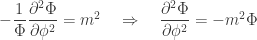
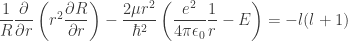
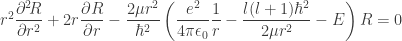
Hence, quantum mechanics. That was one of the mysteries the forefathers of QM tried to solve — how come atoms are stable when all our current physics tells us they shouldn’t be? Fortunately, a century later, we already have a fully developed theory of QM. The motion of a single electron with effective mass moving in the vicinity of a static particle of opposite charge is determined by the time-dependent Schrödinger equation of motion:

Since the Coulomb potential doesn’t depend on time explicitly, we can look for a separated solution in the form of:

The temporal part of the solution is just a periodic complex exponential. The time-independent Schrödinger equation for the spatial part, and the equation we need to solve, is:

One look at the potential tells us that this problem exhibits a spherical symmetry. Spherical coordinates might hence be in order. We will express the vector in terms of the radial coordinate (distance from origin) , and two angles and . The potential written is these coordinates is trivial. The differential operator is a bit more complicated. We can look up the form of the Laplace operator in spherical coordinates on Wikipedia. The equation becomes:

Wow, now that’s a mouthful. Thankfully, there are no mixed derivatives, and we can thus hope to obtain a solution by separating variables. We will use the following Ansatz for the wave function :

At the same time, let us multiply both sides of the equation by , and divide by the factor in front of the square bracket:

When we now divide both sides by the wave function :

we see that solely the third term depends on the azimuth angle $\theta$ and, moreover, it depends only on the azimuth angle!

Azimuthal Equation

We move the term that depends on to the right side of the equals sign:

What we are saying is that something that only depends on has to be equal to another thing that is a function of two other, completely independent variables. The only way this can hold is if both sides are constant. We can call this constant anything, but let us choose the label :

This is a trivial differential equation, the solution of which is a complex exponential. Exponential, because the function remains the same under derivation, and complex, because of the change of sign upon deriving it twice. Hence:

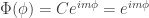
We don’t need to worry about normalization yet, so the constant factor is set to one. The constant is called the magnetic quantum number. Since any solution must be symmetric with respect to a rotation of 360°, the magnetic quantum number is an integer.

Polar Equation

Let us go back to the Schrödinger equation, in which we replace the azimuthal term with the constant :

We can divide by , and separate the terms that depend on the radial and polar coordinates:

Just like before, both sides are equal despite being functions of mutually independent coordinates. As a consequence, they must both be constant. Once again, we could use any label for this constant, but will prove to be a prescient choice. For the polar angle, we find the following equation:

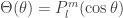Solving this equation is a bit more difficult, and the process is rather technical. The solution is in the form of an associated Legendre polynomial . An interested reader can find a more detailed derivation, for example, here.

One thing to note: in the solution, the satisfaction of a convergence criterion requires that be any positive integer, including 0. We call it, somewhat confusingly, the azimuthal, or orbital quantum number. Moreover, the solution of the polar equation establishes a connection between the magnetic quantum number and the orbital quantum number :

---

The azimuth and polar parts of the solution together form the so-called spherical harmonics :

Apart from the normalization factor, a spherical harmonic is just the product of the two angular parts of the solution, and hence the final solution of the hydrogen problem can be written as:

Radial Equation

Finally, lets us solve the part of the equation that depends on the radial coordinate :

Rearranging the terms, we get:

We can expand the differential operator:

and divide by :

Now, the commonly adopted procedure lies in evaluating the long range limit separately. For large , the terms proportional to or can be neglected, and hence:

Since the energy of bound states is chosen to be negative, the solution of the equation in the above limit is a linear combination of real exponentials. To avoid divergence for large , only the decreasing exponential is selected:

Next, the rest of the radial solution is assumed to be a power series:

Plugging this into the radial equation, and forcing the series to eventually terminate, we can find (a) the solution consisting of associated Laguerre polynomials , (b) the principal quantum number , and (c) the expression for the energy . As this text is getting quite long already, and all this can be found in much more detail in any proper quantum mechanics textbook, I will simply wrap up by providing the final solution of the radial equation:

---

The radial solution thus decays exponentially for large , and exhibits an oscillating, polynomial behavior close to the nucleus. When we combine the spherical harmonics that solve the angular part of the problem with the radial solution, we find the following solution of the hydrogen problem:

where is the reduced Bohr radius:

While the solution looks intimidating, most of the complexity lies in the normalization term, and the rather unfamiliar spherical harmonics and Laguerre polynomials. Rest assured that these are well know and thoroughly understood functions.

The energy is given by:

,

where is one Rydberg, or 13.605 eV. The energy spectrum is quantized, and follows an inverse square relation. In this solution, which does not take magnetic and spin effects into consideration, solely the principal quantum number determines the energy of the state. These days, we know that the separation of energy levels determines the frequencies / wavelengths of the lines in the emission or absorption spectrum. However, before there was a theory of quantum mechanics, the realization that the wavelengths corresponding to the emission lines of heated hydrogen follow such simple and elegant mathematical relationship was simply monumental.

Conclusion

I have tried to give a reasonably comprehensive, yet at the same time a relative simple walk-through of the analytical solution to the hydrogen problem. This first part sets the stage for our own efforts to solve the problem numerically. In the second part, we will use a finite difference scheme to find a solution to the radial equation. In the third part, we will address the finite elements method as an alternative to finite differences.

Till then!

Bifurcation Diagram in OpenGL

Last month we took a look at one of the most famous fractals — the Mandelbrot set. However, there is another fractal that deserves to be mentioned in the same breath. A fractal that appears to be deceivingly simple in its formulation. And yet, one could argue it started chaos theory! Of course, I am talking about the bifurcation diagram. What is even more fascinating, both the bifurcation diagram and the Mandelbrot set are intimately related with each other! Like last time, we will start with a gentle introduction, and then proceed to visualize the fractal using a simple OpenGL program.

Bifurcations? What are those?

Before we answer this question, we need to first talk about the logistic function, or the logistic map. All around us we can observe phenomena exhibiting two antagonistic features competing between each other. The classic example is that of a population of herbivores. The larger the population in a given year, the more offspring is born. Therefore, the size of the population next year must be a directly proportional to its current size. However, the larger the population, the more competition there is for finite resources. Food, or living space, are limited. And thus there will be a second feature trying to oppose the increase of the population size. One of the simplest functions (or rather maps / recursive relations as we’re dealing with discrete values) devised to describe such phenomena is the logistic equation:

where in our analogy, and are the current and future population sizes expressed as a fraction of the maximum population, and is some parameter, presumably related to the actual dynamics of the observed system.

What does this logistic map tell us about future projections of the population size? We could repeatedly apply the recursive relation, and observe the behavior. For example, let’s choose, say, , and try out several starting population sizes (again, expressed as a number between 0 and 1 representing the fraction of the population with respect to the maximum size). The logistic map predicts the following evolution of population size:

We see that regardless of the starting population, our choice of the parameter leads to a unique asymptotic population size. So, let’s fix the starting population, and try different values for :

Previously, we saw that leads to a single asymptotic value. And so do and , too. However, starting from a certain value of , we observe not one asymptotic value, but rather two values between which the population oscillates!

Now, if we were to plot for each the asymptotic value(s), we would see that the line in the diagram splits, or bifurcates, like this:

For each we plot the asymptotic value(s) of the population after some number of iterations. The colored points correspond to the choices of adopted previously.

In fact, we were to keep going, for an even higher choice of the parameter , there would be eventually 4 asymptotic values. And then 8. 16. Until…

1, 2, 4, 8, 16, … ?!

Chaos!

The Algorithm

For each value of :

1. Repeatedly evaluate the logistic map with any starting value a certain number of times to achieve convergence
2. Draw all asymptotic values

Now that’s trivial!

OpenGL Implementation

Since the algorithm was so simple, let us spice things up by trying something new in OpenGL. In the Mandelbrot set post, we used a fragment shader to perform the algorithm for each pixel. At variance, here we only need to apply the algorithm for each value of (point on the horizontal axis) once. Hence, a fragment shader might not really be appropriate here. A vertex shader is also out of the question — after all, we do not know how many vertices (asymptotic values) there will be, even though the GPU needs to be given the list of vertices beforehand. Is there some other kind of shader?

Yes! After the vertex shader executes for each vertex, and before the fragment shader executes for each fragment (~pixel), the geometry shader runs on each primitive. The primitives are just the elementary shapes OpenGL operates with — points, lines, and triangles. A geometry shader can manipulate the primitives defined by the vertices it receives from the vertex shader. It can not only modify the properties of existing primitives, but it can create (emit) additional ones!

So, here’s the deal: we start with a line of points across the screen representing the horizontal axis, the values of the parameter . The trivial vertex shader sends each primitive (point) to the geometry shader. Here we execute our algorithm. For each asymptotic value, we emit a new point at the appropriate vertical coordinate.

---

Unlike in the post on the Mandelbrot set, I will not go into too much detail regarding the general structure of the program. After all, the vast majority of the code is either identical or only exhibits minor modifications. The code in its entirety can be found at the very bottom of this post. Here, we will only discuss the shaders and the most relevant parts of the main file.

As mentioned above, we first set up the array of points, represented by two number, the horizontal and vertical coordinates. We spread the points in a line, one point per each pixel in the horizontal direction, ranging from -1 to +1:

File “main.cpp”:

int main()
{
    ...

    const int num_points = screen_width;
    float vertices[2 * num_points]{};
    for (int i = 0; i < num_points; ++i)
    {
        vertices[2 * i] = -1.0f + 2.0f * (float)i / (float)num_points;
    }

    ...

The main loop of our program looks like this:

int main()
{
    ...
    while (!glfwWindowShouldClose(window))
    {
        process_input(window);
        glClearColor(0.2f, 0.0f, 0.2f, 1.0f);
        glClear(GL_COLOR_BUFFER_BIT | GL_DEPTH_BUFFER_BIT);

        countFPS();

        our_shader.useShader();
        our_shader.set_float("zoom", zoom);
        our_shader.set_float("shift_x", shift_x);
        our_shader.set_float("shift_r", shift_r);

        glBindVertexArray(VAO);
        glDrawArrays(GL_POINTS, 0, num_points);
        glfwSwapBuffers(window);
        glfwPollEvents();
	}
    ...

The process_input() function is practically identical to the one we implemented last month. Just like before, we set the uniform variables in response to the user input. Then, we draw num_points points along the horizontal line. Or at least, that is what the (trivial) vertex shader receives:

File “shader.vert”

#version 330 core
layout (location = 0) in vec2 position;

void main()
{
    gl_Position = vec4(position, 0.0, 1.0);
}

The location of each vertex / point is simply forwarded to the geometry shader. Since we used only two coordinates the describe the points, we have to bolster gl_Position with two more components.

Now to the meat and potatoes of the program — the geometry shader:

File “shader.geom”:

#version 330 compatibility
#define MAX_VERTICES 256

layout(points) in;
layout(points, max_vertices=MAX_VERTICES) out;

uniform float shift_r;
uniform float shift_x;
uniform float zoom;

float update_x(float x, float r)
{
    return r * x * (1.0f - x);
}

void bifurcate(float r, float zoom, float x_shift)
{
    // initial guess
    float x = 0.5f;

    // throw away first N values in the series
    for (int i = 0; i < 2 * MAX_VERTICES; ++i)
    {
        x = update_x(x, r);
    }

    // emit point only if it lands inside viewspace
    int num_emited = 0;

    while (num_emited < MAX_VERTICES)
    {
        x = update_x(x, r);

        float pos = (x - x_shift) / zoom;

        if (pos <= -1.0f && pos <= 1.0f)
        {
            num_emited++;
            gl_Position = gl_in[0].gl_Position + vec4(0.0f, pos, 0.0f, 0.0f);
            EmitVertex();
            EndPrimitive();
        }
    }
}

The function update_x() is our logistic map. The bifurcate() function first calls it a certain number of times. This is to ensure that more-or-less converged asymptotic values are obtained. Next, we start counting the number of emitted (extra) points. There is a hardware limit on the number of vertices a geometry shader can emit processing a single primitive. For my GPU, this value is 256. I believe that this is the lowest value guaranteed by manufacturers, but you may have to reduce this even further. We will iterate the logistic map until we have obtained MAX_VERTICES valid vertices. A vertex shall be valid if it lies on the screen. After all, why bother spending our limited MAX_VERTICES budget on vertices that ultimately won’t be drawn to the screen? Each emitted vertex is shifted vertically by an amount proportional to the value obtained from the logistic map, and scaled/shifted so as to implement user controls in the vertical direction.

Finally, the main() function simply calls bifurcate():

...
void main()
{	
	float r = zoom * gl_in[0].gl_Position.x + shift_r;

	bifurcate(r, zoom, shift_x);
}  

Note how we scale and shift the parameter to “simulate” the panning and zooming in the horizontal direction.

Finally the newly created points are fed to the fragment shader, which, again, is trivial:

File “shader.frag”:

#version 330 core
out vec4 fragment_color;

void main()
{
    fragment_color = vec4(1.0f, 1.0f, 1.0f, 1.0f);
}

We choose to draw all points in white. Boring, I know.

---

As discussed, you can find the whole code below. For now, let’s compile and run our OpenGL program with the above shaders:

Conclusion

I hope we can all appreciate the above animation despite the horrible quality a .gif offers. One can see both the chaotic distribution of the individual points, as well as the fractal, ordered nature of the diagram as a whole. While the logistic map is one of the simplest and most commonly presented function that results in a bifurcation diagram, I was amazed to learn that any function with a “single bump” results in a very similar diagram of its own. In fact, regardless of the function, the distance between subsequent bifurcations follows the same ratio! This, to me, was mind blowing. If you want to learn more, check out the Feigenbaum constants.

---

For your convenience, I’ve added all project files below.

File “main.cpp”:

#include <iostream>
#include <stdlib.h>
#include <string>
#include <math.h>

#include <GL\glew.h>
#include <GLFW\glfw3.h>
#include <GLM\glm.hpp>
#include <GLM\gtc\matrix_transform.hpp>
#include <GLM\gtc\type_ptr.hpp>

#include "Shader.h"

int screen_width{ 1920};
int screen_height{ 1080 };

int num_frames{};
float last_time{};
float zoom{ 1.0f };
float shift_x{  0.5f };
float shift_r{  1.0f };

void framebuffer_size_callback(GLFWwindow * window, int width, int height)
{
    glViewport(0, 0, width, height);
}

void process_input(GLFWwindow * window)
{
    if (glfwGetKey(window, GLFW_KEY_ESCAPE) == GLFW_PRESS)
    {
        glfwSetWindowShouldClose(window, true);
    }

    if (glfwGetKey(window, GLFW_KEY_UP) == GLFW_PRESS)
    {
        shift_x = shift_x + 0.03f * zoom;
        if (shift_x > 4.0f / zoom)
        {
            shift_x = 4.0f / zoom;
        }
    }

    if (glfwGetKey(window, GLFW_KEY_DOWN) == GLFW_PRESS)
    {
        shift_x = shift_x - 0.03f * zoom;
        if (shift_x < 0.0f)
        {
            shift_x = 0.0f;
        }
    }

    if (glfwGetKey(window, GLFW_KEY_LEFT) == GLFW_PRESS)
    {
        shift_r = shift_r - 0.03f * zoom;
        if (shift_r < -4.0f)
        {
            shift_r = -4.0f;
        }
    }

    if (glfwGetKey(window, GLFW_KEY_RIGHT) == GLFW_PRESS)
    {
        shift_r = shift_r + 0.03f * zoom;
        if (shift_r > 4.0f)
        {
            shift_r = 4.0f;
        }
    }

    if (glfwGetKey(window, GLFW_KEY_LEFT_SHIFT) == GLFW_PRESS)
    {
        zoom = zoom * 1.04f;
        if (zoom > 10.0f)
        {
            zoom = 10.0f;
        }
    }

    if (glfwGetKey(window, GLFW_KEY_LEFT_CONTROL) == GLFW_PRESS)
    {
        zoom = zoom * 0.96f;
        if (zoom < 0.00001f)
        {
            zoom = 0.00001f;
        }
    }
}

void countFPS()
{
    double current_time = glfwGetTime();
    num_frames++;
    if (current_time - last_time >= 1.0)
    {
        std::cout << 1000.0 / num_frames << "ms / frame\n";
        num_frames = 0;
        last_time += 1.0;
    }
}

int main()
{
    glfwInit();
    glfwWindowHint(GLFW_CONTEXT_VERSION_MAJOR, 3);
    glfwWindowHint(GLFW_CONTEXT_VERSION_MINOR, 3);
    glfwWindowHint(GLFW_OPENGL_PROFILE, GLFW_OPENGL_CORE_PROFILE);

    GLFWwindow * window = glfwCreateWindow(screen_width, screen_height, "Mandelbrot", NULL, NULL);

    if (window == nullptr)
    {
        std::cout << "Failed to create GLFW window!\n";
        glfwTerminate();
        return -1;
    }

    glfwMakeContextCurrent(window);

    if (glewInit())
    {
        std::cout << "Failed initializing GLEW\n";
    }

    glViewport(0, 0, screen_width, screen_height);
    glfwSetFramebufferSizeCallback(window, framebuffer_size_callback);
    
    Shader our_shader("Shaders/shader.vert", "Shaders/shader.geom", "Shaders/shader.frag");

    const int num_points = screen_width;

    float vertices[2 * num_points]{};
    for (int i = 0; i < num_points; ++i)
    {
        vertices[2 * i] = -1.0f + 2.0f * (float)i / (float)num_points;
    }

    unsigned int VAO, VBO;
    glGenVertexArrays(1, &VAO);
    glGenBuffers(1, &VBO);

    glBindVertexArray(VAO);

    glBindBuffer(GL_ARRAY_BUFFER, VBO);
    glBufferData(GL_ARRAY_BUFFER, sizeof(vertices), vertices, GL_STATIC_DRAW);

    glVertexAttribPointer(0, 2, GL_FLOAT, GL_FALSE, 2 * sizeof(float), (void*)0);
    glEnableVertexAttribArray(0);

    glBindBuffer(GL_ARRAY_BUFFER, 0);
    glBindVertexArray(0);

    last_time = glfwGetTime();

    glEnable(GL_DEPTH_TEST);
    while (!glfwWindowShouldClose(window))
    {
        glClearColor(0.2f, 0.0f, 0.2f, 1.0f);
        glClear(GL_COLOR_BUFFER_BIT | GL_DEPTH_BUFFER_BIT);

        process_input(window);
        countFPS();

        our_shader.use_shader();
        our_shader.set_float("zoom", zoom);
        our_shader.set_float("shift_x", shift_x);
        our_shader.set_float("shift_r", shift_r);

        glBindVertexArray(VAO);
        
        glDrawArrays(GL_POINTS, 0, num_points);

        glfwSwapBuffers(window);
        glfwPollEvents();
    }

    glDeleteVertexArrays(1, &VAO);
    glDeleteBuffers(1, &VBO);

    glfwTerminate();
    return 0;
}

File “shader.vert”:

#version 330 core
layout (location = 0) in vec2 position;

void main()
{
    gl_Position = vec4(position, 0.0, 1.0);
}

File “shader.geom”

#version 330 compatibility
#define MAX_VERTICES 256

layout(points) in;
layout(points, max_vertices=MAX_VERTICES) out;

uniform float shift_r;
uniform float shift_x;
uniform float zoom;

float update_x(float x, float r)
{
    return r * x * (1.0f - x);
}

void bifurcate(float r, float zoom, float x_shift)
{
    // initial guess
    float x = 0.5f;

    // throw away first N values in the series
    for (int i = 0; i < 2 * MAX_VERTICES; ++i)
    {
        x = update_x(x, r);
    }

    // emit point only if it lands inside viewspace
    int num_emited = 0;

    while (num_emited < MAX_VERTICES)
    {
        x = update_x(x, r);

        float pos = (x - x_shift) / zoom;

        if (pos <= -1.0f && pos <= 1.0f)
        {
            num_emited++;
            gl_Position = gl_in[0].gl_Position + vec4(0.0f, pos, 0.0f, 0.0f);
            EmitVertex();
            EndPrimitive();
        }
    }
}

void main()
{	
	float r = zoom * gl_in[0].gl_Position.x + shift_r;

	bifurcate(r, zoom, shift_x);
}  

File “shader.frag”:

#version 330 core
out vec4 fragment_color;

void main()
{
    fragment_color = vec4(1.0f, 1.0f, 1.0f, 1.0f);
}

File “Shader.h”:

#pragma once
#include <iostream>
#include <fstream>
#include <sstream>
#include <string>

#include <GL/glew.h>
#include <GLFW/glfw3.h>
#include <GLM/glm.hpp>
#include <GLM/gtc/type_ptr.hpp>

class Shader
{
public:
	unsigned int program_ID;
	Shader(const char * vertex_shader_path, const char * fragment_shader_path);
Shader(const char * vertex_shader_path, const char * geometry_shader_path, const char * fragment_shader_path);
	~Shader();

	void use_shader();

	void set_float(const std::string & name, float value) const;
	void set_vec4(const std::string & name, glm::vec4 vec) const;

private:
	std::string read_shader_file(const char * file_path);
	void add_shader(unsigned int program, const char * shader_path, GLenum shader_type);
};

File “Shader.cpp”:

#include "Shader.h"

Shader::Shader(const char * vertex_shader_path, const char * fragment_shader_path)
{
	program_ID = glCreateProgram();

	add_shader(program_ID, vertex_shader_path, GL_VERTEX_SHADER);
	add_shader(program_ID, fragment_shader_path, GL_FRAGMENT_SHADER);

	glLinkProgram(program_ID);

	int success;
	char error_message[512];
	glGetProgramiv(program_ID, GL_LINK_STATUS, &success);
	if (!success)
	{
		glGetProgramInfoLog(program_ID, 512, nullptr, error_message);
		std::cout << "Error linking shader program: " << error_message << "\n";
	}
}

Shader::Shader(const char * vertex_shader_path, const char * geometry_shader_path, const char * fragment_shader_path)
{
	program_ID = glCreateProgram();

	add_shader(program_ID, vertex_shader_path, GL_VERTEX_SHADER);
	add_shader(program_ID, geometry_shader_path, GL_GEOMETRY_SHADER);
	add_shader(program_ID, fragment_shader_path, GL_FRAGMENT_SHADER);

	glLinkProgram(program_ID);

	int success;
	char error_message[512];
	glGetProgramiv(program_ID, GL_LINK_STATUS, &success);
	if (!success)
	{
		glGetProgramInfoLog(program_ID, 512, nullptr, error_message);
		std::cout << "Error linking shader program: " << error_message << "\n";
	}
}

Shader::~Shader()
{
	if (program_ID != 0)
	{
		glDeleteProgram(program_ID);
		program_ID = 0;
	}
}

void Shader::use_shader()
{
	glUseProgram(program_ID);
}


std::string Shader::read_shader_file(const char * file_path)
{
	std::string code;
	std::ifstream shader_file(file_path, std::ios::in);

	if (!shader_file)
	{
		std::cout << "Failed to open shader file: " << file_path << "\n";
		return "";
	}

	std::string line = "";
	while (std::getline(shader_file, line))
	{
		code.append(line + '\n');
	}
		
	shader_file.close();
	return code;
}

void Shader::add_shader(unsigned int program, const char * shader_path, GLenum shader_type)
{
	std::string shader_string = read_shader_file(shader_path);

	const GLchar * code[1];
	code[0] = shader_string.c_str();

	GLint code_length[1];
	code_length[0] = strlen(shader_string.c_str());

	unsigned int shader;
	int success;
	char error_message[512];

	shader = glCreateShader(shader_type);
	glShaderSource(shader, 1, code, code_length);
	glCompileShader(shader);

	glGetShaderiv(shader, GL_COMPILE_STATUS, &success);
	if (!success)
	{
		glGetShaderInfoLog(shader, 512, nullptr, error_message);
		std::cout << "Error compiling shader: " << error_message << "\n";
		std::cout << "Shader location: " << shader_path << "\n";
	}

	glAttachShader(program, shader);
}

void Shader::set_float(const std::string & name, float value) const
{
	glUniform1f(glGetUniformLocation(program_ID, name.c_str()), value);
}

void Shader::set_vec4(const std::string & name, glm::vec4 vec) const
{
	glUniform4f(glGetUniformLocation(program_ID, name.c_str()), vec.x, vec.y, vec.z, vec.w);
}

Visualizing the Mandelbrot Set Using OpenGL, Part 2

Last time we have written an OpenGL program that enables us to draw a visual representation of the famous Mandelbrot set. Unfortunately, we could not behold it in its full glory. The final image was dark, monotone, and far too static — when what we want is a way to investigate all the tiny details hiding yet more details in all their fractal beauty. Hence, today we will improve our program. First, we implement simple controls that allow us to move around the complex plane and zoom in on anything that catches our eye in real time. Second, we will improve the visuals by introducing dynamic ranges rendered in different colors, so that not a single feature of the fractal goes unnoticed.

Controls

We here implement a simple control functionality that allows the view to zoom in and out, as well as to move around the complex number plane. The actual implementation might seem counter-intuitive at first. First of all, instead of actually moving the camera, it is usually the world itself that is moved around with respect to a static camera. Furthermore, in our case we actually won’t even move the world around! The two triangles acting as a backdrop for our fractal will remain static. What we will change instead is the subset, the rectangle, of the complex number plane, that we feed to our Mandelbrot algorithm. 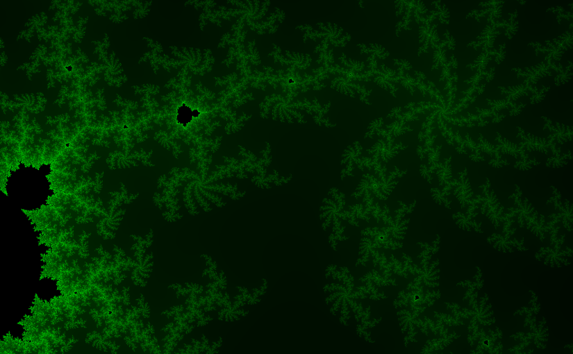For example, if we want to move right, we simply increase the real part of the value evaluated in the algorithm. Likewise, zooming in can be understood as scaling all the values in the complex plane by some factor smaller than one. The end effect will look like we move the camera back and forth, but we won’t need to deal with all the complexities of setting up everything from cameras and projections to model and view transformations.

We add a function in our “main.cpp” file that registers and processes user input. This function will be called at every frame of our simulation, and the processed input it receives will be sent to the shader program.

In file “main.cpp”:

float center_x{ 0.0f };
float center_y{ 0.0f };
float zoom{ 1.0 };

void process_input(GLFWwindow * window)
{
    if (glfwGetKey(window, GLFW_KEY_ESCAPE) == GLFW_PRESS)
    {
        glfwSetWindowShouldClose(window, true);
    }

    if (glfwGetKey(window, GLFW_KEY_UP) == GLFW_PRESS)
    {
        center_y = center_y + 0.005f * zoom;
        if (center_y > 1.0f)
        {
            center_y = 1.0f;
	}
    }

    if (glfwGetKey(window, GLFW_KEY_DOWN) == GLFW_PRESS)
    {
        center_y = center_y - 0.005f * zoom;
        if (center_y < -1.0f)
        {
            center_y = -1.0f;
        }
    }

    if (glfwGetKey(window, GLFW_KEY_LEFT) == GLFW_PRESS)
    {
        center_x = center_x - 0.005f * zoom;
        if (center_x < -1.0f)
        {
            center_x = -1.0f;
        }
    }

    if (glfwGetKey(window, GLFW_KEY_RIGHT) == GLFW_PRESS)
    {
        center_x = center_x + 0.005f * zoom;
        if (center_x > 1.0f)
        {
            center_x = 1.0f;
        }
    }

    if (glfwGetKey(window, GLFW_KEY_LEFT_SHIFT) == GLFW_PRESS)
    {
        zoom = zoom * 1.02f;
        if (zoom > 1.0f)
        {
            zoom = 1.0f;
        }
    }

    if (glfwGetKey(window, GLFW_KEY_LEFT_CONTROL) == GLFW_PRESS)
    {
        zoom = zoom * 0.98f;
        if (zoom < 0.00001f)
        {
            zoom = 0.00001f;
        }
    }
}

...

First, we make it so that pressing the escape key closes the window. Next, we handle the up and down arrows. Pressing them increases or decreases the center of the coordinate, respectively, which in our case corresponds to moving along the complex direction. The handling of the left and right arrow keys should be self-explanatory in the light of the above. Note that we scale the “speed” of translation by our zoom value. If we did not, then moving around while zoomed out would be too slow, while any details would flick by in an instant when zoomed in. Finally, we address zooming in and out. Here, we keep multiplying the zoom value at the press of the corresponding key. Again, this ensures that the act of zooming feels the same regardless of how zoomed in we are currently.

Now that we processed the user’s input, we need to communicate the value of center_x, center_y, and zoom to the shader program in charge of rendering the fractal. We do this through uniform variables. If you look at the Shader class in the previous post, you will note that we already implement the functionality of sending data to the GPU. We simply declare a uniform variable in a shader file, and then tell OpenGL that we want to associate this uniform variable with a variable in our current program. In our case, in each iteration of the render loop we send the values of center_x, center_y, and zoom to their appropriately named uniform counterparts in the fragment shader.

File “main.cpp”:

...

void main()
{
    ...

    while (!glfwWindowShouldClose(window))
    {
        ...

        process_input(window);
        
        our_shader.use_shader();
        our_shader.set_float("zoom", zoom);
        our_shader.set_float("center_x", center_x);
        our_shader.set_float("center_y", center_y);

        ...
    }
}

...

---

Now we just need to make sure our fragment shader considers a rectangle of the complex plane centered at center_x, center_y and appropriately zoomed in. First, we declare the uniform variables corresponding to those in the main program. Then, we modify the get_iterations() function as follows.

In file “shader.frag”:

...

uniform float center_x;
uniform float center_y;
uniform float zoom;

int get_iterations()
{
	float real = ((gl_FragCoord.x / 1080.0f - 0.5f) * zoom + center_x) * 4.0f;
	float imag = ((gl_FragCoord.y / 1080.0f - 0.5f) * zoom + center_y) * 4.0f;

	int iterations = 0;
	float const_real = real;
	float const_imag = imag;

	while (iterations < MAX_ITERATIONS)
	{
		float tmp_real = real;
		real = (real * real - imag * imag) + const_real;
		imag = (2.0f * tmp_real * imag) + const_imag;
		
		float dist = real * real + imag * imag;

		if (dist > 4.0f)
			break;

		++iterations;
	}
	return iterations;
}

...

That’s it! We can now fly around the fractal, zooming in on any detail that catches our eye!

Color Ranges

Next, we work on the visuals. The issue with the current program is that the color of each pixel only corresponds to the absolute number of iterations of the Mandelbrot algorithm. Areas that differ just by a few iterations are rendered in practically the same color. Thus as we progressively zoom in, some of the detail remains hidden due to low contrast. Instead, what we want to do is find out what the lowest and the highest number of iterations corresponding to the rendered view is. Then we can effectively build a histogram of all values between the bounds, and color each bin, or range, in different colors. This preserves the same contrast at any zoom level.

The implementation requires that we somehow move the information of the number of iterations from the GPU to our program. We could set up an array of data, a buffer, fill it with the necessary information and then work with that. However, there is already a buffer we can, so to say, hijack! We encode the information about the number of iterations in the depth buffer. You can imagine the depth buffer as an array of floating point values between 0 and 1 representing the distance of each fragment from the camera. Since our shaders do not require this information, we can fill the depth buffer with the number of iterations (or rather the fraction of achieved iterations with respect to their maximum value). In practice, this just means specifying gl_FragDepth() as an output parameter, and assigning it the appropriate value:

In file “shader.frag”:

...

out float gl_FragDepth;

vec4 return_color()
{
    int iter = get_iterations();
    if (iter == MAX_ITERATIONS)
    {
        gl_FragDepth = 0.0f;
        return vec4(0.0f, 0.0f, 0.0f, 1.0f);
    }

    float iterations = float(iter) / MAX_ITERATIONS;
    gl_FragDepth = iterations;

    ...
}

...

We process the number of iterations encoded in the depth buffer, calculate the appropriate iteration ranges for the various colors, and send this information back to the GPU. To do this, we declare another uniform variable, color_ranges, this time a vec4. We proceed as follows: for each fragment we calculate the number of iterations of the algorithm. If the corresponding point is in the set, this number is MAX_ITERATIONS, we color the fragment black and output a value of 0. Else, we take the relative number of iterations and look in which range it falls. For instance, if it’s between the first and second value of the vector color_ranges, we color the fragment by mixing color_0 and color_1 with a ratio corresponding to the position of the iteration count within the appropriate bounds. The whole function looks like this:

In file “shader.frag”:

...

out float gl_FragDepth;
uniform vec4 color_ranges;

vec4 return_color()
{
    int iter = get_iterations();
    if (iter == MAX_ITERATIONS)
    {
        gl_FragDepth = 0.0f;
        return vec4(0.0f, 0.0f, 0.0f, 1.0f);
    }

    float iterations = float(iter) / MAX_ITERATIONS;
    gl_FragDepth = iterations;

    vec4 color_0 = vec4(0.0f, 0.0f, 0.0f, 1.0f);
    vec4 color_1 = vec4(0.0f, 0.2f, 0.5f, 1.0f);
    vec4 color_2 = vec4(1.0f, 0.8f, 0.0f, 1.0f);
    vec4 color_3 = vec4(1.0f, 0.0f, 0.4f, 1.0f);

    float fraction = 0.0f;
    if (iterations < color_ranges[1])
    {
        fraction = (iterations - color_ranges[0]) / (color_ranges[1] - color_ranges[0]);
        return mix(color_0, color_1, fraction);
    }
    else if(iterations < color_ranges[2])
    {
        fraction = (iterations - color_ranges[1]) / (color_ranges[2] - color_ranges[1]);
        return mix(color_1, color_2, fraction);
    }
    else
    {
        fraction = (iterations - color_ranges[2]) / (color_ranges[3] - color_ranges[2]);
        return mix(color_2, color_3, fraction);
    }
}

...

---

The last thing to do is to actually compute the iteration ranges. We implement the function find_ranges() that takes the iteration data as a standard vector of floats, and returns the vec4 representing the color ranges:

In file “main.cpp”:

...

glm::vec4 find_ranges(std::vector<float> & data)
{
    std::sort(data.begin(), data.end());
    int lowest = 0;
    while (data[lowest] == 0.0f)
    {
        ++lowest;
    }

    int size = data.size();
    int length = size - lowest;
    glm::vec4 ranges = glm::vec4( data[lowest], data[lowest + length * 3 / 4 - 1], data[lowest + length * 7 / 8 - 1], data[size - 1] );
    return ranges;
}

We first sort all data. This leaves us with some amount of zeroes (which correspond to pixels in the Mandelbrot set), and non-zero values. The pixels that belong to the set should remain black, so we want to ignore all zero values. We search for the first non-zero value at index lowest. The first bound is this lowest non-zero value. We place the next bound to the value at around three quarters in the remaining sorted iterations. The next bound is placed at around seven eighths, and the last one represents the highest iteration value present. I chose these values by trial and error, you may experiment with them yourself and find better ranges.

In the main() function we first set up the initial ranges. Then, in the render loop, we send the vector holding the ranges to the corresponding uniform variable. After we draw the fractal, we retrieve the iteration values for each fragment using glReadPixels(), and then pass them to our find_ranges() function, to have the ranges ready for the next frame.

In file “main.cpp”:

...

int main()
{
    ...

    std::vector<float> pixel_data(screen_width * screen_height, 0.0f);
    glm::vec4 ranges = glm::vec4(0.0001f, 0.33333f, 0.66667f, 1.00f);

    while (!glfwWindowShouldClose(window))
    {
        ...

        our_shader.set_vec4("color_ranges", ranges);

        ...

        glReadPixels(0, 0, screen_width, screen_height, GL_DEPTH_COMPONENT, GL_FLOAT, pixel_data.data());
        ranges = find_ranges(pixel_data);
    }

    ...
}

That’s it!

Conclusion

We have improved our original program by implementing controls, which allow us to move around and zoom in on the fractal, and by playing around with the colors and their intensity, which allows us to preserve the same contrast regardless of what part of the complex plane we are observing. The following is a very crude representation of our program — I had to stitch an animated .gif from individual screenshots. Kind of lame, I know. But you can imagine how much cooler our actual program is.

Until next time!

---

All files are reproduced below.

File “main.cpp”:

#include <iostream>
#include <stdlib.h>
#include <string>
#include <math.h>
#include <algorithm>
#include <vector>

#include <GL\glew.h>
#include <GLFW\glfw3.h>
#include <GLM\glm.hpp>
#include <GLM\gtc\matrix_transform.hpp>
#include <GLM\gtc\type_ptr.hpp>

#include "Shader.h"

int screen_width{ 1080 };
int screen_height{ 1080 };

int num_frames{};
float last_time{};
float center_x{ 0.0f };
float center_y{ 0.0f };
float zoom{ 1.0 };

float vertices[] = 
{
//    x      y      z   
    -1.0f, -1.0f, -0.0f,
     1.0f,  1.0f, -0.0f,
    -1.0f,  1.0f, -0.0f,
     1.0f, -1.0f, -0.0f
};

unsigned int indices[] = 
{
//  2---,1
//  | .' |
//  0'---3
    0, 1, 2,
    0, 3, 1
};


void framebuffer_size_callback(GLFWwindow * window, int width, int height)
{
    glViewport(0, 0, width, height);
}


void process_input(GLFWwindow * window)
{
    if (glfwGetKey(window, GLFW_KEY_ESCAPE) == GLFW_PRESS)
    {
        glfwSetWindowShouldClose(window, true);
    }

    if (glfwGetKey(window, GLFW_KEY_UP) == GLFW_PRESS)
    {
        center_y = center_y + 0.01f * zoom;
        if (center_y > 1.0f)
        {
            center_y = 1.0f;
        }
    }

    if (glfwGetKey(window, GLFW_KEY_DOWN) == GLFW_PRESS)
    {
        center_y = center_y - 0.01f * zoom;
        if (center_y < -1.0f)
        {
            center_y = -1.0f;
        }
    }

    if (glfwGetKey(window, GLFW_KEY_LEFT) == GLFW_PRESS)
    {
        center_x = center_x - 0.01f * zoom;
        if (center_x < -1.0f)
        {
            center_x = -1.0f;
        }
    }

    if (glfwGetKey(window, GLFW_KEY_RIGHT) == GLFW_PRESS)
    {
        center_x = center_x + 0.01f * zoom;
        if (center_x > 1.0f)
        {
            center_x = 1.0f;
        }
    }

    if (glfwGetKey(window, GLFW_KEY_LEFT_SHIFT) == GLFW_PRESS)
    {
        zoom = zoom * 1.04f;
        if (zoom > 1.0f)
        {
            zoom = 1.0f;
        }
    }

    if (glfwGetKey(window, GLFW_KEY_LEFT_CONTROL) == GLFW_PRESS)
    {
        zoom = zoom * 0.96f;
        if (zoom < 0.00001f)
        {
            zoom = 0.00001f;
        }
    }
}

void countFPS()
{
    double current_time = glfwGetTime();
    num_frames++;
    if (current_time - last_time >= 1.0)
    {
        std::cout << 1000.0 / num_frames << "ms / frame\n";
        num_frames = 0;
        last_time += 1.0;
    }
}

glm::vec4 find_ranges(std::vector<float> & data)
{
    std::sort(data.begin(), data.end());
    int lowest = 0;
    while (data[lowest] == 0.0f)
    {
        ++lowest;
    }

    int size = data.size();
    int length = size - lowest;
    glm::vec4 ranges = glm::vec4( data[lowest], data[lowest + length * 3 / 4 - 1], data[lowest + length * 7 / 8 - 1], data[size - 1] );
    return ranges;
}

int main()
{
    glfwInit();
    glfwWindowHint(GLFW_CONTEXT_VERSION_MAJOR, 3);
    glfwWindowHint(GLFW_CONTEXT_VERSION_MINOR, 3);
    glfwWindowHint(GLFW_OPENGL_PROFILE, GLFW_OPENGL_CORE_PROFILE);

    GLFWwindow * window = glfwCreateWindow(screen_width, screen_height, "Mandelbrot", NULL, NULL);

    if (window == nullptr)
    {
        std::cout << "Failed to create GLFW window!\n";
        glfwTerminate();
        return -1;
    }

    glfwMakeContextCurrent(window);

    if (glewInit())
    {
        std::cout << "Failed initializing GLEW\n";
    }

    glViewport(0, 0, screen_width, screen_height);
    glfwSetFramebufferSizeCallback(window, framebuffer_size_callback);
    
    Shader our_shader("Shaders/shader.vert", "Shaders/shader.frag");

    unsigned int VAO, VBO, EBO;
    glGenVertexArrays(1, &VAO);
    glGenBuffers(1, &VBO);
    glGenBuffers(1, &EBO);

    glBindVertexArray(VAO);

    glBindBuffer(GL_ARRAY_BUFFER, VBO);
    glBufferData(GL_ARRAY_BUFFER, sizeof(vertices), vertices, GL_STATIC_DRAW);

    glBindBuffer(GL_ELEMENT_ARRAY_BUFFER, EBO);
    glBufferData(GL_ELEMENT_ARRAY_BUFFER, sizeof(indices), indices, GL_STATIC_DRAW);

    glVertexAttribPointer(0, 3, GL_FLOAT, GL_FALSE, 3 * sizeof(float), (void*)0);
    glEnableVertexAttribArray(0);

    glBindBuffer(GL_ARRAY_BUFFER, 0);
    glBindVertexArray(0);

    last_time = glfwGetTime();

    glEnable(GL_DEPTH_TEST);

    std::vector<float> pixel_data(screen_width * screen_height, 0.0f);
    glm::vec4 ranges = glm::vec4(0.0001f, 0.33333f, 0.66667f, 1.00f);

    while (!glfwWindowShouldClose(window))
    {
        glClearColor(0.2f, 0.0f, 0.2f, 1.0f);
        glClear(GL_COLOR_BUFFER_BIT | GL_DEPTH_BUFFER_BIT);

        process_input(window);
        countFPS();

        our_shader.use_shader();
        our_shader.set_float("zoom", zoom);
        our_shader.set_float("center_x", center_x);
        our_shader.set_float("center_y", center_y);
        our_shader.set_vec4("color_ranges", ranges);

        glBindVertexArray(VAO);
        
        glDrawElements(GL_TRIANGLES, 6, GL_UNSIGNED_INT, 0);

        glfwSwapBuffers(window);
        glfwPollEvents();

        glReadPixels(0, 0, screen_width, screen_height, GL_DEPTH_COMPONENT, GL_FLOAT, pixel_data.data());
        ranges = find_ranges(pixel_data);
    }

    glDeleteVertexArrays(1, &VAO);
    glDeleteBuffers(1, &VBO);
    glDeleteBuffers(1, &EBO);

    glfwTerminate();
    return 0;
}

File “shader.frag”:

#version 330 core
in vec4 gl_FragCoord;

out vec4 fragColor;
out float gl_FragDepth;

uniform float center_x;
uniform float center_y;
uniform float zoom;
uniform vec4 color_ranges;

#define MAX_ITERATIONS 600

int get_iterations()
{
    float real = ((gl_FragCoord.x / 1080.0f - 0.5f) * zoom + center_x) * 4.0f;
    float imag = ((gl_FragCoord.y / 1080.0f - 0.5f) * zoom + center_y) * 4.0f;

    int iterations = 0;
    float const_real = real;
    float const_imag = imag;

    while (iterations < MAX_ITERATIONS)
    {
        float tmp_real = real;
        real = (real * real - imag * imag) + const_real;
        imag = (2.0 * tmp_real * imag) + const_imag;
        
        float dist = real * real + imag * imag;

        if (dist > 4.0)
            break;

        ++iterations;
    }
    return iterations;
}


vec4 return_color()
{
    int iter = get_iterations();
    if (iter == MAX_ITERATIONS)
    {
        gl_FragDepth = 0.0f;
        return vec4(0.0f, 0.0f, 0.0f, 1.0f);
    }

    float iterations = float(iter) / MAX_ITERATIONS;
    gl_FragDepth = iterations;

    vec4 color_0 = vec4(0.0f, 0.0f, 0.0f, 1.0f);
    vec4 color_1 = vec4(0.0f, 0.2f, 0.5f, 1.0f);
    vec4 color_2 = vec4(1.0f, 0.8f, 0.0f, 1.0f);
    vec4 color_3 = vec4(1.0f, 0.0f, 0.4f, 1.0f);

    float fraction = 0.0f;
    if (iterations < color_ranges[1])
    {
        fraction = (iterations - color_ranges[0]) / (color_ranges[1] - color_ranges[0]);
        return mix(color_0, color_1, fraction);
    }
    else if(iterations < color_ranges[2])
    {
        fraction = (iterations - color_ranges[1]) / (color_ranges[2] - color_ranges[1]);
        return mix(color_1, color_2, fraction);
    }
    else
    {
        fraction = (iterations - color_ranges[2]) / (color_ranges[3] - color_ranges[2]);
        return mix(color_2, color_3, fraction);
    }
}

void main()
{
    fragColor = return_color();
}

File “shader.vert”:

#version 330 core
layout (location = 0) in vec3 pos;

void main()
{
    gl_Position = vec4(pos.xyz, 1.0);
}

File “Shader.h”:

#pragma once
#include <iostream>
#include <fstream>
#include <sstream>
#include <string>

#include <GL/glew.h>
#include <GLFW/glfw3.h>
#include <GLM/glm.hpp>
#include <GLM/gtc/type_ptr.hpp>

class Shader
{
public:
	unsigned int program_ID;
	Shader(const char * vertex_shader_path, const char * fragment_shader_path);
	~Shader();

	void use_shader();

	void set_float(const std::string & name, float value) const;
	void set_vec4(const std::string & name, glm::vec4 vec) const;

private:
	std::string read_shader_file(const char * file_path);
	void add_shader(unsigned int program, const char * shader_path, GLenum shader_type);
};

File “Shader.cpp”:

#include "Shader.h"

Shader::Shader(const char * vertex_shader_path, const char * fragment_shader_path)
{
	program_ID = glCreateProgram();

	add_shader(program_ID, vertex_shader_path, GL_VERTEX_SHADER);
	add_shader(program_ID, fragment_shader_path, GL_FRAGMENT_SHADER);

	glLinkProgram(program_ID);

	int success;
	char error_message[512];
	glGetProgramiv(program_ID, GL_LINK_STATUS, &success);
	if (!success)
	{
		glGetProgramInfoLog(program_ID, 512, nullptr, error_message);
		std::cout << "Error linking shader program: " << error_message << "\n";
	}
}

Shader::~Shader()
{
	if (program_ID != 0)
	{
		glDeleteProgram(program_ID);
		program_ID = 0;
	}
}

void Shader::use_shader()
{
	glUseProgram(program_ID);
}


std::string Shader::read_shader_file(const char * file_path)
{
	std::string code;
	std::ifstream shader_file(file_path, std::ios::in);

	if (!shader_file)
	{
		std::cout << "Failed to open shader file: " << file_path << "\n";
		return "";
	}

	std::string line = "";
	while (std::getline(shader_file, line))
	{
		code.append(line + '\n');
	}
		
	shader_file.close();
	return code;
}

void Shader::add_shader(unsigned int program, const char * shader_path, GLenum shader_type)
{
	std::string shader_string = read_shader_file(shader_path);

	const GLchar * code[1];
	code[0] = shader_string.c_str();

	GLint code_length[1];
	code_length[0] = strlen(shader_string.c_str());

	unsigned int shader;
	int success;
	char error_message[512];

	shader = glCreateShader(shader_type);
	glShaderSource(shader, 1, code, code_length);
	glCompileShader(shader);

	glGetShaderiv(shader, GL_COMPILE_STATUS, &success);
	if (!success)
	{
		glGetShaderInfoLog(shader, 512, nullptr, error_message);
		std::cout << "Error compiling shader: " << error_message << "\n";
		std::cout << "Shader location: " << shader_path << "\n";
	}

	glAttachShader(program, shader);
}

void Shader::set_float(const std::string & name, float value) const
{
	glUniform1f(glGetUniformLocation(program_ID, name.c_str()), value);
}

void Shader::set_vec4(const std::string & name, glm::vec4 vec) const
{
	glUniform4f(glGetUniformLocation(program_ID, name.c_str()), vec.x, vec.y, vec.z, vec.w);
}

Visualizing the Mandelbrot Set Using OpenGL, Part 1

In this two-part series I will show you how to visualize the Mandelbrot set using modern OpenGL. In this first part, we set up everything in order to render the scene and write a shader that draws a visual representation of the famous fractal. In a future post we will implement some elementary controls that will enable us to move around and zoom in & out, and we will also play around with the shaders to make the fractal look more stunning.

The Mandelbrot Set

Take a complex number . Feed it to the function , where the initial value of . Take the result of this (let’s call it ) and plug it back into the function. Repeat with , , ad infinitum. Is the modulus of , its distance from the origin of the complex plane, below ? If yes, then is in the Mandelbrot set!

To give an example, let’s choose :

and so on and so forth. One can see that has a modulus of , and , hence is not in the Mandelbrot set.

What about ? Then we get the series , , , . Clearly, this series tends to grow, but only very slowly, approaching the value . And since this number is smaller than , is in the Mandelbrot set.

There are two interesting observations to make here. First, the Mandelbrot set is a fractal — a “self-similar” shape with a complex topology. You can keep zooming in on a fractal and you will never find some clear boundary. Some fractals are nice and repeating. Instead, although this fractal exhibits some repeating themes, it is closely linked to chaos. It’s impossible to say whether two close numbers belong to the set or not, as the complex numbers along it’s boundary are chaotically being thrown around, either remaining within a distance of from the origin or being flung out.

Second, even the numbers which do not belong in the set show this chaotic behavior. One choice of might cross after the fifth iteration, like we have seen above. And another , infinitesimally larger or smaller, might take ten billion iterations of the process before .

---

So, to visualize the Mandelbrot set, we implement the following algorithm:

For each in the complex plane:

1. Calculate
2. If then stop and return
3. If go to 1. and repeat

Additionally, we must implement some sort of maximum number of iterations above which we interrupt the algorithm and assume the number is in the set. If we don’t, and is indeed in the Mandelbrot set, we simply keep iterating forever!

Implementation

I will not go into detail regarding the setup of the OpenGL work environment in Visual Studio (my IDE of choice), nor will I discuss the basics of OpenGL here. First of all, I am no expert, and therefore my tutorial might not be of real value to many of you. Second, there are already plenty of amazing resources available on the web covering these topics in great detail. I heartily recommend LearnOpenGL, a freely accessible series of tutorials covering everything from the basics of OpenGL to advanced shader techniques. Likewise, I’d like to highlight the Udemy course Computer Graphics with Modern OpenGL and C++. While this one is not for free, with the seasonal 95+% sales on Udemy you can get it for a few bucks sooner or later.

---

Let’s start with setting up our main file. Following LearnOpenGL, we include several libraries that enable us to interact with the graphics processor. We also instantiate a few helper variables, notably the dimensions of the screen. Finally, we create a simple array of floats vertices that will represent the coordinates of the four corners of the rectangle filling the screen, and an array of integers indices which indexes the above vertices defining two triangles:

File “main.cpp”:

#include <iostream>
#include <stdlib.h>
#include <string>

#include <GL\glew.h>
#include <GLFW\glfw3.h>
#include <GLM\glm.hpp>
#include <GLM\gtc\matrix_transform.hpp>
#include <GLM\gtc\type_ptr.hpp>

#include "Shader.h"

int screen_width{ 1080 };
int screen_height{ 1080 };

int num_frames{ 0 };
float last_time{ 0.0f };

float vertices[] = 
{
//    x      y      z   
    -1.0f, -1.0f, -0.0f,
     1.0f,  1.0f, -0.0f,
    -1.0f,  1.0f, -0.0f,
     1.0f, -1.0f, -0.0f
};

unsigned int indices[] = 
{
//  2---,1
//  | .' |
//  0'---3
    0, 1, 2,
    0, 3, 1
};

...

Next, we implement two quick functions. One will allow us to resize the window. The other one measures the time it takes to render a frame. Each render loop we increment the frame count, and each second we print out the time it took to render one frame on average, in milliseconds. We could take the inverse of this number and have a regular FPS counter, but talking about the time per frame rather than frames per time is often more meaningful from the point of view of optimizing our code:

...

void framebuffer_size_callback(GLFWwindow * window, int width, int height)
{
    glViewport(0, 0, width, height);
}

void countFPS()
{
    double current_time = glfwGetTime();
    num_frames++;
    if (current_time - last_time >= 1.0)
    {
        std::cout << 1000.0 / num_frames << "ms / frame\n";
        num_frames = 0;
        last_time += 1.0;
    }
}

...

In the main() function we first set up a window in preparation for our rendering (as I said, I won’t go into details explaining these steps; take a look at LearnOpenGL to learn more):

...

int main()
{
    glfwInit();
    glfwWindowHint(GLFW_CONTEXT_VERSION_MAJOR, 3);
    glfwWindowHint(GLFW_CONTEXT_VERSION_MINOR, 3);
    glfwWindowHint(GLFW_OPENGL_PROFILE, GLFW_OPENGL_CORE_PROFILE);

    GLFWwindow * window = glfwCreateWindow(screen_width, screen_height, "Mandelbrot", NULL, NULL);

    if (window == nullptr)
    {
        std::cout << "Failed to create GLFW window!\n";
        glfwTerminate();
        return -1;
    }

    glfwMakeContextCurrent(window);

    if (glewInit())
    {
        std::cout << "Failed initializing GLEW\n";
    }

    glViewport(0, 0, screen_width, screen_height);
    glfwSetFramebufferSizeCallback(window, framebuffer_size_callback);

    last_time = glfwGetTime();

    ...
}

Once a window is set up, we make the data representing our rectangle available to the GPU. This is done via vertex array objects (VAOs), which in turn rely on vertex buffer objects (VBOs) and element buffer objects (EBOs). First, a VAO is created — it represents all data related to the vertices to be drawn. Instead of passing around custom structs or large arrays, we simply refer to different VAOs when we want to draw the corresponding vertices. We copy the coordinates of these vertices into a buffer: the VBO. If we worked with more complicated 3D scenes, we might have a second VBO for the normal vectors, and another one for texture coordinates. For our purpose here, one VBO is enough. And likewise, we copy the indices into another buffer, the EBO, as the indices represent the actual elements to be drawn:

int main()
{
    ...

    unsigned int VAO, VBO, EBO;
    glGenVertexArrays(1, &VAO);
    glGenBuffers(1, &VBO);
    glGenBuffers(1, &EBO);

    glBindVertexArray(VAO);

    glBindBuffer(GL_ARRAY_BUFFER, VBO);
    glBufferData(GL_ARRAY_BUFFER, sizeof(vertices), vertices, GL_STATIC_DRAW);

    glBindBuffer(GL_ELEMENT_ARRAY_BUFFER, EBO);
    glBufferData(GL_ELEMENT_ARRAY_BUFFER, sizeof(indices), indices, GL_STATIC_DRAW);

    glVertexAttribPointer(0, 3, GL_FLOAT, GL_FALSE, 3 * sizeof(float), (void*)0);
    glEnableVertexAttribArray(0);

    glBindBuffer(GL_ARRAY_BUFFER, 0);
    glBindVertexArray(0);

    ...
}

Finally, we set up our shaders. The corresponding class Shader is implemented in the files “Shader.h” and “Shader.cpp”, which you can find at the bottom of this post. Again, it’s beyond the scope of this post to delve into how any of this is done. What we care about here is that we only need a single line to run our shader later on:

int main()
{
    ...

    Shader our_shader("shader.vert", "shader.frag");

    ...
}

---

With everything set up properly, we can enter the render loop. The following code will be executed every single frame. What we need to do is tell OpenGL to 1) eraze whatever was shown last frame, 2) update the FPS counter, 3) use our shader, and 4) render the rectangle that represents the background, on which the shader draws the fractal:

int main()
{
    ...

    while (!glfwWindowShouldClose(window))
    {
        glClearColor(0.0f, 0.0f, 0.0f, 1.0f);
        glClear(GL_COLOR_BUFFER_BIT | GL_DEPTH_BUFFER_BIT);

        countFPS();

        our_shader.use_shader();

        glBindVertexArray(VAO);
        glDrawElements(GL_TRIANGLES, 6, GL_UNSIGNED_INT, 0);

        glfwSwapBuffers(window);
        glfwPollEvents();
    }

    glDeleteVertexArrays(1, &VAO);
    glDeleteBuffers(1, &VBO);
    glDeleteBuffers(1, &EBO);

    glfwTerminate();
    return 0;
}

The Shader

Shaders are files written in a C-like language that get executed by the graphical processing unit. OpenGL uses a pipeline of several shader programs, each of which takes care of a different aspect of rendering the desired scene. There can be more types of shader files, but for our intents and purposes we only need two: the vertex shader and the fragment shader.

The vertex shader is the first to be executed. It operates on each vertex. Vertex shaders can do such things as move vertices around, or change their properties. We only render two triangles that form a rectangle filling the view. There is no additional work to be done with them, so our vertex shader file “shader.vert” can remain very simple:

File “shader.vert”:

#version 330 core
layout (location = 0) in vec3 pos;

void main()
{
	gl_Position = vec4(pos.xyz, 1.0);
}

The pos variable corresponds to the VBO with the vertices we have previously bound to location 0. These coordinates are then passed on unmodified to an internal OpenGL variable that tells the GPU where the vertex is. In essence, we just need to tell the GPU where the buffer with the vertex coordinates is.

---

The fragment shader needs to be more complicated. One may imagine that fragments represent the actual pixels, even though in reality they do not. Basically, the fragment shader is executed for each fragment (or pixel) on the scene and returns the color of that pixel. What we will do is we will use the position of the fragment in the rendered view as the coordinates in complex space that we will feed to our Mandelbrot algorithm. The fragment shader starts with telling the GPU that we want to take the position of the fragment as an input, and output the final color value. Then, we define a function that actually returns the number of iterations of the Mandelbrot set algorithm:

File “shader.frag”:

#version 330 core
in vec4 gl_FragCoord;

out vec4 frag_color;

#define MAX_ITERATIONS 500

int get_iterations()
{
    float real = (gl_FragCoord.x / 1080.0 - 0.5) * 4.0;
    float imag = (gl_FragCoord.y / 1080.0 - 0.7) * 4.0;

    int iterations = 0;
    float const_real = real;
    float const_imag = imag;

    while (iterations < MAX_ITERATIONS)
    {
        float tmp_real = real;
        real = (real * real - imag * imag) + const_real;
        imag = (2.0 * tmp_real * imag) + const_imag;
		
        float dist = real * real + imag * imag;
        
        if (dist > 4.0)
	    break;

        ++iterations;
    }
    return iterations;
}

...

As there is no native support for complex numbers, we handle the real and imaginary parts separately by defining real and imag. The position of the fragment in gl_FragCoord is expressed through integers starting from 0 all the way to the width and height of the rendered view. We divide these coordinates by the width and the height to get a real and a complex number, respectively, between 0 and 1. We then shift them a bit to center them more or less around the origin, and then “zoom in” by scaling by a factor of four. The view should now correspond to a part of the complex plane in size and centered around zero (with a slight shift in the negative real direction).

The real and imag parts are then repeatedly fed into the Mandelbrot set algorithm, repeating the process up to MAX_ITERATIONS defined at the beginning of the file. If the complex number “escapes” the set, we return the number of iterations it took it to do so. If even after all those iterations it is inside the set, we assume it remains there for good, and return MAX_ITERATIONS.

Next, we use the count of the iterations as a way to color the fragment via the return_color() function. If the iteration count is MAX_ITERATIONS we color the fragment black. These parts of the image represent the actual numbers in the complex plane that belong to the Mandelbrot set. All other fragments are colored green, the intensity of the color being directly proportional to the number of iterations of the algorithm it took to discard that point:

...

vec4 return_color()
{
    int iter = get_iterations();
    if (iter == MAX_ITERATIONS)
    {
        gl_FragDepth = 0.0f;
        return vec4(0.0f, 0.0f, 0.0f, 1.0f);
    }

    float iterations = float(iter) / MAX_ITERATIONS;	
    return vec4(0.0f, iterations, 0.0f, 1.0f);
}

void main()
{
    frag_color = return_color();
}

The main() function of the fragment shader is then trivial.

Result

We compile our program and run it. And this is what we get:

The Mandelbrot set in all its beauty. Or not really. The image is kind of noisy, too dark. And little detail can be seen around the set. Not to mention, it would probably be nicer if we could zoom in and move around.

We can “zoom in” by manually modifying the variables real and imag in the fragment shader. And we can change to colors by varying how the intensity depends on the number of iterations. Unfortunately, we still have a non-interactive rendering. All these issues will be solved in the second part. 🙂

Until then!

---

File “main.cpp”:

#include <iostream>
#include <stdlib.h>
#include <string>

#include <GL\glew.h>
#include <GLFW\glfw3.h>
#include <GLM\glm.hpp>
#include <GLM\gtc\matrix_transform.hpp>
#include <GLM\gtc\type_ptr.hpp>

#include "Shader.h"

int screen_width{ 1080 };
int screen_height{ 1080 };

int num_frames{ 0 };
float last_time{ 0.0f };

float vertices[] = 
{
//    x      y      z   
    -1.0f, -1.0f, -0.0f,
     1.0f,  1.0f, -0.0f,
    -1.0f,  1.0f, -0.0f,
     1.0f, -1.0f, -0.0f
};

unsigned int indices[] = 
{
//  2---,1
//  | .' |
//  0'---3
    0, 1, 2,
    0, 3, 1
};


void framebuffer_size_callback(GLFWwindow * window, int width, int height)
{
    glViewport(0, 0, width, height);
}

void countFPS()
{
    double current_time = glfwGetTime();
    num_frames++;
    if (current_time - last_time >= 1.0)
    {
        std::cout << 1000.0 / num_frames << "ms / frame\n";
        num_frames = 0;
        last_time += 1.0;
    }
}

int main()
{
    glfwInit();
    glfwWindowHint(GLFW_CONTEXT_VERSION_MAJOR, 3);
    glfwWindowHint(GLFW_CONTEXT_VERSION_MINOR, 3);
    glfwWindowHint(GLFW_OPENGL_PROFILE, GLFW_OPENGL_CORE_PROFILE);

    GLFWwindow * window = glfwCreateWindow(screen_width, screen_height, "Mandelbrot", NULL, NULL);

    if (window == nullptr)
    {
        std::cout << "Failed to create GLFW window!\n";
        glfwTerminate();
        return -1;
    }

    glfwMakeContextCurrent(window);

    if (glewInit())
    {
        std::cout << "Failed initializing GLEW\n";
    }

    glViewport(0, 0, screen_width, screen_height);
    glfwSetFramebufferSizeCallback(window, framebuffer_size_callback);

    unsigned int VAO, VBO, EBO;
    glGenVertexArrays(1, &VAO);
    glGenBuffers(1, &VBO);
    glGenBuffers(1, &EBO);

    glBindVertexArray(VAO);

    glBindBuffer(GL_ARRAY_BUFFER, VBO);
    glBufferData(GL_ARRAY_BUFFER, sizeof(vertices), vertices, GL_STATIC_DRAW);

    glBindBuffer(GL_ELEMENT_ARRAY_BUFFER, EBO);
    glBufferData(GL_ELEMENT_ARRAY_BUFFER, sizeof(indices), indices, GL_STATIC_DRAW);

    glVertexAttribPointer(0, 3, GL_FLOAT, GL_FALSE, 3 * sizeof(float), (void*)0);
    glEnableVertexAttribArray(0);

    glBindBuffer(GL_ARRAY_BUFFER, 0);
    glBindVertexArray(0);

    Shader our_shader("shader.vert", "shader.frag");

    last_time = glfwGetTime();

    glEnable(GL_DEPTH_TEST);

    while (!glfwWindowShouldClose(window))
    {
        glClearColor(0.2f, 0.0f, 0.2f, 1.0f);
        glClear(GL_COLOR_BUFFER_BIT | GL_DEPTH_BUFFER_BIT);

        countFPS();

        our_shader.use_shader();
        glBindVertexArray(VAO);
		
        glDrawElements(GL_TRIANGLES, 6, GL_UNSIGNED_INT, 0);

        glfwSwapBuffers(window);
        glfwPollEvents();

    }

    glDeleteVertexArrays(1, &VAO);
    glDeleteBuffers(1, &VBO);
    glDeleteBuffers(1, &EBO);

    glfwTerminate();
    return 0;
}

File “shader.vert”:

#version 330 core
layout (location = 0) in vec3 pos;

void main()
{
	gl_Position = vec4(pos.xyz, 1.0);
}

File “shader.frag”:

#version 330 core
in vec4 gl_FragCoord;

out vec4 frag_color;

#define MAX_ITERATIONS 500

int get_iterations()
{
    float real = ((gl_FragCoord.x / 1080.0 - 0.5) * zoom + center_x) * 5.0;
    float imag = ((gl_FragCoord.y / 1080.0 - 0.5) * zoom + center_y) * 5.0;

    int iterations = 0;
    float const_real = real;
    float const_imag = imag;

    while (iterations < MAX_ITERATIONS)
    {
        float tmp_real = real;
        real = (real * real - imag * imag) + const_real;
        imag = (2.0 * tmp_real * imag) + const_imag;
		
        float dist = real * real + imag * imag;
        
        if (dist > 4.0)
	    break;

        ++iterations;
    }
    return iterations;
}

vec4 return_color()
{
    int iter = get_iterations();
    if (iter == MAX_ITERATIONS)
    {
        gl_FragDepth = 0.0f;
        return vec4(0.0f, 0.0f, 0.0f, 1.0f);
    }

    float iterations = float(iter) / MAX_ITERATIONS;	
    return vec4(0.0f, iterations, 0.0f, 1.0f);
}

void main()
{
    frag_color = return_color();
}

File “Shader.h”:

#pragma once
#include <iostream>
#include <fstream>
#include <sstream>
#include <string>

#include <GL/glew.h>
#include <GLFW/glfw3.h>
#include <GLM/glm.hpp>
#include <GLM/gtc/type_ptr.hpp>

class Shader
{
public:
	unsigned int program_ID;
	Shader(const char * vertex_shader_path, const char * fragment_shader_path);
	~Shader();

	void use_shader();

	void set_float(const std::string & name, float value) const;
	void set_vec4(const std::string & name, glm::vec4 vec) const;

private:
	std::string read_shader_file(const char * file_path);
	void add_shader(unsigned int program, const char * shader_path, GLenum shader_type);
};

File “Shader.cpp”:

#include "Shader.h"

Shader::Shader(const char * vertex_shader_path, const char * fragment_shader_path)
{
	program_ID = glCreateProgram();

	add_shader(program_ID, vertex_shader_path, GL_VERTEX_SHADER);
	add_shader(program_ID, fragment_shader_path, GL_FRAGMENT_SHADER);

	glLinkProgram(program_ID);

	int success;
	char error_message[512];
	glGetProgramiv(program_ID, GL_LINK_STATUS, &success);
	if (!success)
	{
		glGetProgramInfoLog(program_ID, 512, nullptr, error_message);
		std::cout << "Error linking shader program: " << error_message << "\n";
	}
}

Shader::~Shader()
{
	if (program_ID != 0)
	{
		glDeleteProgram(program_ID);
		program_ID = 0;
	}
}

void Shader::use_shader()
{
	glUseProgram(program_ID);
}


std::string Shader::read_shader_file(const char * file_path)
{
	std::string code;
	std::ifstream shader_file(file_path, std::ios::in);

	if (!shader_file)
	{
		std::cout << "Failed to open shader file: " << file_path << "\n";
		return "";
	}

	std::string line = "";
	while (std::getline(shader_file, line))
	{
		code.append(line + '\n');
	}
		
	shader_file.close();
	return code;
}

void Shader::add_shader(unsigned int program, const char * shader_path, GLenum shader_type)
{
	std::string shader_string = read_shader_file(shader_path);

	const GLchar * code[1];
	code[0] = shader_string.c_str();

	GLint code_length[1];
	code_length[0] = strlen(shader_string.c_str());

	unsigned int shader;
	int success;
	char error_message[512];

	shader = glCreateShader(shader_type);
	glShaderSource(shader, 1, code, code_length);
	glCompileShader(shader);

	glGetShaderiv(shader, GL_COMPILE_STATUS, &success);
	if (!success)
	{
		glGetShaderInfoLog(shader, 512, nullptr, error_message);
		std::cout << "Error compiling shader: " << error_message << "\n";
		std::cout << "Shader location: " << shader_path << "\n";
	}

	glAttachShader(program, shader);
}

void Shader::set_float(const std::string & name, float value) const
{
	glUniform1f(glGetUniformLocation(program_ID, name.c_str()), value);
}


void Shader::set_vec4(const std::string & name, glm::vec4 vec) const
{
	glUniform4f(glGetUniformLocation(program_ID, name.c_str()), vec.x, vec.y, vec.z, vec.w);
}

Band Edge Alignment from Density Functional Theory

Today, we will be talking about the alignment of the band gap edges of semiconductors with respect to vacuum — as calculated with density functional theory (DFT). If you are in a rush, feel free to skip to the end, where I present a short python script to perform the projection of a .cube file and the band alignment procedure. If you’ve got some time on your hands, or want to understand what is it we’re trying to do, enjoy the read!

Short Introduction

Let’s start with a simple atom, say, hydrogen. Solving the time independent Schrödinger equation for the single electron of the hydrogen atom yields a set of discrete eigenvalues (energy levels) and corresponding eigenvectors (in this case, orbitals). The discrete nature of the energy spectrum is a feature of any bound quantum system, whether we talk about an electron bound to a nucleus, a photon confined between two mirrors, or even a quasiparticle trapped in a potential well. I will leave the detailed discussion of the hydrogen atom for a later time. For now, we just need to acknowledge that the energy spectrum of a hydrogen atom consists of discrete values, with the electron in the ground state occupying the lowest possible level.

Next, consider a molecule. Something large, like an organic one, for example. One may imagine that all the atomic orbitals interact with those of other atoms. The corresponding energy levels split and shift, forming so-called bonding and anti-bonding orbitals. Instead of just a few far apart values, a molecular energy spectrum contains bunches of values stemming from the splitting and rearranging of the underlying atomic energy levels.

Now, increase the size of the molecule — to the point it becomes a solid. There are so many atoms and electrons, the bunched up discrete values simply merge, forming literal bands in the energy spectrum. See the below figure for a visual representation of the above:

Finally, just like with the hydrogen atom, the electrons occupy the available bands from bottom up. It may happen that the highest occupied orbital (HOMO, where the M stands for ‘molecular’, but that is the convention I adopt here) corresponds to an energy value within a band. In that case, many other achievable states exist, with just a slightly higher energy. Applying an electric field, for example, speeds up the electrons, giving them a little bit more energy, shifting their energy levels slightly higher. Such materials are called metals.

However, it may so happen that the HOMO of a particular material is at the very top of a band, separated from the lowest unoccupied orbital (LUMO) by a sizable gap in the energy spectrum, the band gap. In that case, the electrons cannot easily accept the extra energy in the form of electric fields. If they were to speed up, they would acquire more energy, but there is no available state with just a tad more energy. The closest one is on the other side of the gap. Hence the response of these materials to electric fields or electromagnet radiation (light) will be very different than that of metals. These materials are called insulators, or if the gap is relatively small, semiconductors.

It is this gap that we are interested in. In semiconductors, we call the highest occupied band the valence band, whereas the lowest unoccupied band is called the conduction band. The exact positions of the edges of these bands are very important for many applications, such as electronic components, lasers, or the catalysis of chemical reactions.

---

Given an atomic structure, we can find the electronic ground state using density functional theory, or DFT. Unfortunately, DFT relies on some approximations that make it impossible to compare the absolute results with experiment. In general, it is only DFT energy differences that may be safely compared with measurable quantities. For example, the total energy of a helium atom evaluated using DFT is not physically meaningful — it depends on the adopted functional and on other, more subtle details of implementation. However, the separation between the two lowest energy levels of that helium atom can be calculated with DFT, and it compares favorably with experiment.

What does it mean for our problem? We can solve the electronic structure of a solid using DFT, and acquire the energy spectrum, including the HOMO and the LUMO levels. While their difference (the band gap) is physically meaningful (to an extent), their absolute positions are not. Therefore, we need a scheme that allows us to align the position of the HOMO and LUMO (the edges of the valence and conduction band, respectively) with respect to some sort of absolute, physical reference. In this case, we choose vacuum as our reference.

Alignment Procedure

We will align the position of the band edges as follows:

First, we perform a bulk semiconductor calculation, and determine the alignment between the average bulk electrostatic potential and the band edges.

Second, we carry out a simulation of a semiconductor slab interfaced with vacuum. We compute the distance between the average electrostatic potential inside the slab, and in the vacuum.

Combining the results of these two calculations allows us to finally align the band edges with respect to vacuum via the average electrostatic potential.

---

I am using CP2K, a mixed Gaussian / plane wave DFT code. Like most other DFT software packages, it allows one to run geometry and cell optimization calculations. So, here is a step-by-step explanation of the calculations that need to be performed:

1. Cell optimization to find optimal atom configuration and lattice parameters of the bulk material
2. Single point energy calculation on the final configuration to print out the electrostatic potential, and the positions of the HOMO and LUMO levels
3. Using the optimized geometry and lattice parameters, build a supercell with a vacuum interface, and optimize the geometry
4. Single point energy calculation of the final supercell to again obtain the electrostatic potential across the cell and the positions of the HOMO and LUMO levels

Implementation

CP2K prints out the electrostatic potential in the Gaussian cube file format. Once our simulations are complete, the first thing we need to do is take the cube files, parse the data, and project the potential along the direction perpendicular to the interface. We will do the same for the bulk cell, even though CP2K uses the average electrostatic potential across the whole cell as the zero reference for the energy scale. This means that as long as we deal with a bulk calculation, the position of the energy levels is given with respect to the average electrostatic potential which is set to zero, and hence, in principle, no extra alignment has to be carried out here. But other codes might not use the same reference and the bulk alignment may be necessary as well.

The cube file format is a human-readable file format that represents data using an orthogonal volumetric grid. Basically, the value for each point $latex(x, y, z)$ is listed in a text file. The file format is described here.

---

Let us start with the base class that we will later specialize into the bulk and interface child classes:

import scipy as sp

BOHR_TO_A = 0.5291772
HARTREE_TO_EV = 27.211396132

class Cube:
    def __init__(self, filename, fermi_level, band_gap):
        self.filename = filename
        self.name = filename.split('.')[0]
        self.valence_band = fermi_level
        self.conduction_band = fermi_level + band_gap

        if filename.split('.')[-1] == 'cube':
            self.parse_cube_file()
            self.project_along_z()
            self.write_projection_file()
        
        elif filename.split('.')[-1] == 'dat':
            self.parse_projection_file()
        
        else:
            error_message = 'Format of {:s} not supported'.format(self.filename)
            raise Exception(error_message)
            

We initialize a Cube object by providing the location of an input file, the Fermi level (HOMO), and the width of the band gap. Since cube files are generally quite large, and we don’t need all that information, we will make it possible to parse them, process them, and write a simple text file (.dat extension) with only the necessary data.

The cube file can be parsed as follows:

class Cube:
    ...
    def parse_cube_file(self):
        with open(self.filename, 'r') as f:
            raw_data = f.readlines()
            
        self.natoms = int(raw_data[2].split()[0])
        self.nx, self.ny, self.nz = [int(line.split()[0]) for line in raw_data[3:6]]
        self.dx, self.dy, self.dz = [float(line.split()[i + 1]) for i, line in enumerate(raw_data[3:6])]
        self.A = self.nx * self.dx * BOHR_TO_A
        self.B = self.ny * self.dy * BOHR_TO_A
        self.C = self.nz * self.dz * BOHR_TO_A
        
        self.data = []
        for line in raw_data[self.natoms + 6:]:
            self.data.extend(float(x) for x in line.split())

        self.potential = sp.zeros((self.nx, self.ny, self.nz))
        for i in range(self.nx):
            for j in range(self.ny):
                for k in range(self.nz):
                    self.potential[i, j, k] = self.data[i * self.ny * self.nz + j * self.nz + k] * HARTREE_TO_EV
        
        print('Cube file {:s} parsed\n'.format(self.filename))

We read the header and set some internal variables, like the number of points, size of the cell, etc. I prefer working with angstroms, hence we do the appropriate conversions. Next, we unroll the data, which is written in rows of six values, into a single long column. Finally, we set up potential, an array, to hold the values of the electrostatic potential on the real space grid.

Once the cube file is parsed, we can proceed to project the potential along the direction perpendicular to the interface. Here we assume the slab is periodic in the and directions, with being oriented perpendicular to the surface. As potential is an array, we can simply sum up along the direction parallel with the interface, and divide by the number of points in each such plane to obtain the average of the projected electrostatic potential:

class Cube:
    ...   
    def project_along_z(self):
        self.projection_z = sp.sum(sp.sum(self.potential, axis=0), axis=0)
        self.projection_z /= (self.nx * self.ny)
    ...

Now that we have condensed the huge cube file (hundreds of MB) into a single array orders of magnitude smaller, we don’t really want to keep parsing the cube file. So we write a text file holding all necessary information, and make it possible to pass this data file as the input of our Cube class:

class Cube:
    ...
    def write_projection_file(self):
        with open(self.name + '.dat', 'w') as f:
            f.write('{:d}\n'.format(self.natoms))
            f.write('{:d} {:d} {:d}\n'.format(self.nx, self.ny, self.nz))
            f.write('{: 10.7f} {: 10.7f} {: 10.7f}\n'.format(self.dx, self.dy, self.dz))
            for value in self.projection_z:
                f.write('{: 8.5f}\n'.format(value))
        
        print('Projection file {:s} written\n'.format(self.name + '.dat'))

    def parse_projection_file(self):
        with open(self.filename, 'r') as f:
            raw_data = f.readlines()
            
        self.natoms = int(raw_data[0].split()[0])
        self.nx, self.ny, self.nz = [int(value) for value in raw_data[1].split()]
        self.dx, self.dy, self.dz = [float(value) for value in raw_data[2].split()]
        self.A = self.nx * self.dx * BOHR_TO_A
        self.B = self.ny * self.dy * BOHR_TO_A
        self.C = self.nz * self.dz * BOHR_TO_A
        
        self.projection_z = sp.zeros(self.nz)
        for i, line in enumerate(raw_data[3:]):
            self.projection_z[i] = float(line.split()[0])
        
        print('Cube file {:s} parsed\n'.format(self.filename))

    ...

The above should be rather self-explanatory.

As a bonus, we write a base method for plotting the projected potential:

class Cube:
    ...
    def plot_projection(self):
        x_axis = sp.linspace(0, self.C, self.nz)
        plt.plot(x_axis, self.projection_z, label=self.name)
        plt.title(self.name)
        plt.legend(loc=3)
        plt.show()

We can demonstrate the operation of this class using a cube file of a vacuum interface. We project the potential, and plot it:

One can see that where the atoms in each crystal plane are located the projected potential dips down, forming sharp troughs. We now need to average this curve over the central region of the slab, and to determine the position of the HOMO and LUMO with respect to the average potential in both the bulk cell and in the vacuum in interface.

---

The base class now prepared, we can create two child classes for the vacuum interface and the bulk system. The Cube_Bulk class might look like this:

class Cube_Bulk(Cube):
    def __init__(self, filename, fermi_level, band_gap):
        super().__init__(filename, fermi_level, band_gap)
    
    def calculate_average_potential(self):
        self.average_potential = sum(self.projection_z) / len(self.projection_z)
    
    def plot_projection(self):
        plt.hlines(self.average_potential, 0.0, self.C)
        plt.hlines(self.valence_band, 0.0, self.C)
        plt.hlines(self.conduction_band, 0.0, self.C)
        super().plot_projection()

As already discussed, in CP2K, the average electrostatic potential across the whole cell is set to zero, and hence this child class is rather pointless. In any case, it is quite simple. There is nothing more to do than to initialize the base class, and then implement the method calculate_average_potential() that computes the average potential. As an extra, we write a quick method to plot the projected potential along the cell. It calls its namesake in the base class, and overlays some horizontal lines to represent the average potential, HOMO and LUMO.

---

The Cube_Interface child class is a tad more complex on account of having to first determine the region in which we average the electrostatic potential. This region should be in the center of the slab, so that we only average over the bulk-like region of the projected potential. We will implement the class as follows:

class Cube_Interface(Cube):
    def __init__(self, filename, fermi_level, band_gap, 
                 start_peak=1, end_peak=3, cutoff=-10.0):
        super().__init__(filename, fermi_level, band_gap)
        self.start_peak = start_peak
        self.end_peak = end_peak
        self.cutoff = cutoff
    
    def find_peaks(self):
        peaks = []
        last_value = self.projection_z[0]
        is_looking_for_minimum = True
        
        for i, value in enumerate(self.projection_z):
            if not is_looking_for_minimum and value > self.cutoff:
                is_looking_for_minimum = True
                
            if is_looking_for_minimum:
                if value > last_value and value < self.cutoff:
                    peaks.append(i - 1)
                    is_looking_for_minimum = False
                    
                last_value = value  
        return peaks
    ...

We initialize using the base class constructor. We pass several extra parameters: which peaks we want to average between, and cutoff, a value required to correctly determine the position of the peaks. We then implement the actual find_peaks() method. The idea is the following — we iterate over the projected potential. Any time we dip below cutoff, we look for a minimum. If we encounter a value of the potential larger than the preceding one we just passed the minimum. We append the index of this minimum to the peaks list. Once all minima are found, the list is returned.

And yes, I call them peaks even though they are the exact opposite. Sue me. See if I care.

Knowing the positions of the peaks corresponding to crystal planes we can now choose a region in the center of the slab and calculate the average electrostatic potential. This is implemented in the calculate_average_potential() method:

class Cube_Interface(Cube):
    ...
    def calculate_average_potential(self):
        peaks = self.find_peaks()
        center_potential = self.projection_z[peaks[self.start_peak] : 
                                             peaks[self.end_peak]]
        self.average_potential = sum(center_potential) / len(center_potential)
        self.vacuum_level = max(self.projection_z)
        
    def plot_projection(self):
        peaks = self.find_peaks()
        start_peak_pos = peaks[self.start_peak] * self.dz * BOHR_TO_A
        end_peak_pos = peaks[self.end_peak] * self.dz * BOHR_TO_A
        plt.hlines(self.average_potential, start_peak_pos, end_peak_pos)
        super().plot_projection()

The bulk-like region is chosen manually by passing the index of the initial and final crystal planes. One could implement some smart way of choosing the center layers. However, sometimes the slab is split, so to speak, due to being wrapped around the periodic cell, in which case it’s much easier to just visually inspect the projected potential and choose the appropriate peaks between which to average.

To help with this visual inspection, we also highlight the averaged-over region using a horizontal line.

---

Finally, it’s time to combine the bulk and the interface objects to determine the overall alignment. We will do this using a quick Alignment class:

class Alignment:
    def __init__(self, bulk, interface):
        self.bulk = bulk
        self.interface = interface
        
        self.name = bulk.name.split('_')[0]
        
        if not self.interface.average_potential:
            self.interface.calculate_average_potential()
            
        if not self.bulk.average_potential:
            self.bulk.calculate_average_potential()
        
        self.calculate_band_edges()
        
    def calculate_band_edges(self):
        vacuum = self.interface.vacuum_level
        valence_band = self.bulk.valence_band - self.bulk.average_potential
        conduction_band = self.bulk.conduction_band - self.bulk.average_potential
        self.adjusted_valence_band = (self.interface.average_potential + valence_band) - vacuum
        self.adjusted_conduction_band = (self.interface.average_potential + conduction_band) - vacuum
        print('Conduction band: {: 5.3f} eV'.format(self.adjusted_conduction_band))
        print('Valence band:    {: 5.3f} eV'.format(self.adjusted_valence_band))

The idea of the alignment process can be more easily understood using the following graphic:

Illustration of the alignment procedure. On the left, the band edges (red) are aligned with respect to the average electrostatic potential (dashed grey). On the right, the average of the electrostatic potential inside the slab (dashed grey) is aligned with respect to the bulk value. Then, the position of the band edges with respect to the electrostatic potential of the interface cell can be determined. And once that is known, one can obtain the alignment with respect to the vacuum potential (black arrows).

We can now parse the cube files, determine the average potential, and combine the bulk and vacuum calculations to obtain the overall alignment:

TiO2_vacuum = Cube_Interface('TiO2_vacuum.cube', -2.655171, 4.606532)
TiO2_vacuum.calculate_average_potential()
TiO2_vacuum.plot_projection()

TiO2_bulk = Cube_Bulk('TiO2_bulk.cube', 4.601682, 4.674498)
TiO2_bulk.calculate_average_potential()
TiO2_bulk.plot_projection()

TiO2 = Alignment(TiO2_bulk, TiO2_vacuum)

And we obtain the values -4.9 eV for the LUMO (or conduction band) and -9.6 eV for the HOMO (or valence band). These values can then be compared with the experimental electron affinity and ionization potential, respectively.

Until next time!

---

Below you will find the whole script:

BOHR_TO_A = 0.5291772
HARTREE_TO_EV = 27.211396132

class Cube:
    def __init__(self, filename, fermi_level, band_gap):
        self.filename = filename
        self.name = filename.split('.')[0]
        self.valence_band = fermi_level
        self.conduction_band = fermi_level + band_gap
        
        if filename.split('.')[-1] == 'cube':
            self.parse_cube_file()
            self.project_along_z()
            self.write_projection_file()
        
        elif filename.split('.')[-1] == 'dat':
            self.parse_projection_file()
        
        else:
            error_message = 'File format of file {:s} not supported'.format(self.filename)
            raise Exception(error_message)
            
    def parse_cube_file(self):
        with open(self.filename, 'r') as f:
            raw_data = f.readlines()
            
        self.natoms = int(raw_data[2].split()[0])
        self.nx, self.ny, self.nz = [int(line.split()[0]) for line in raw_data[3:6]]
        self.dx, self.dy, self.dz = [float(line.split()[i + 1]) for i, line in enumerate(raw_data[3:6])]
        self.A = self.nx * self.dx * BOHR_TO_A
        self.B = self.ny * self.dy * BOHR_TO_A
        self.C = self.nz * self.dz * BOHR_TO_A
        
        self.data = []
        for line in raw_data[self.natoms + 6:]:
            self.data.extend(float(x) for x in line.split())
            
        self.potential = sp.zeros((self.nx, self.ny, self.nz))
        for i in range(self.nx):
            for j in range(self.ny):
                for k in range(self.nz):
                    self.potential[i, j, k] = self.data[i * self.ny * self.nz + j * self.nz + k] * HARTREE_TO_EV
        
        print('Cube file {:s} parsed\n'.format(self.filename))

    def parse_projection_file(self):
        with open(self.filename, 'r') as f:
            raw_data = f.readlines()
            
        self.natoms = int(raw_data[0].split()[0])
        self.nx, self.ny, self.nz = [int(value) for value in raw_data[1].split()]
        self.dx, self.dy, self.dz = [float(value) for value in raw_data[2].split()]
        self.A = self.nx * self.dx * BOHR_TO_A
        self.B = self.ny * self.dy * BOHR_TO_A
        self.C = self.nz * self.dz * BOHR_TO_A
        
        self.projection_z = sp.zeros(self.nz)
        for i, line in enumerate(raw_data[3:]):
            self.projection_z[i] = float(line.split()[0])
        
        print('Cube file {:s} parsed\n'.format(self.filename))
        
    def write_projection_file(self):
        with open(self.name + '.dat', 'w') as f:
            f.write('{:d}\n'.format(self.natoms))
            f.write('{:d} {:d} {:d}\n'.format(self.nx, self.ny, self.nz))
            f.write('{: 10.7f} {: 10.7f} {: 10.7f}\n'.format(self.dx, self.dy, self.dz))
            for value in self.projection_z:
                f.write('{: 8.5f}\n'.format(value))
        
        print('Projection file {:s} written\n'.format(self.name + '.dat'))
    
    def project_along_z(self):
        self.projection_z = sp.sum(sp.sum(self.potential, axis=0), axis=0)
        self.projection_z /= (self.nx * self.ny)
    
    def plot_projection(self):
        x_axis = sp.linspace(0, self.C, self.nz)
        plt.plot(x_axis, self.projection_z, label=self.name)
        plt.title(self.name)
        plt.xlim([min(x_axis), max(x_axis)])
        plt.ylim([min(self.projection_z) - 5, max(self.projection_z) + 5])
        plt.show()
        
class Cube_Interface(Cube):
    def __init__(self, filename, fermi_level, band_gap, start_peak=1, end_peak=3, cutoff=-10.0):
        super().__init__(filename, fermi_level, band_gap)
        self.start_peak = start_peak
        self.end_peak = end_peak
        self.cutoff = cutoff
    
    def find_peaks(self):
        peaks = []
        last_value = self.projection_z[0]
        is_looking_for_minimum = True
        
        for i, value in enumerate(self.projection_z):
            if not is_looking_for_minimum and value > self.cutoff:
                is_looking_for_minimum = True
                
            if is_looking_for_minimum:
                if value > last_value and value < self.cutoff:
                    peaks.append(i - 1)
                    is_looking_for_minimum = False
                    
                last_value = value
            
        return peaks
    
    def calculate_average_potential(self):
        peaks = self.find_peaks()
        center_potential = self.projection_z[peaks[self.start_peak] : peaks[self.end_peak]]
        self.average_potential = sum(center_potential) / len(center_potential)
        self.vacuum_level = max(self.projection_z)
        
    def plot_projection(self):
        peaks = self.find_peaks()
        start_peak_pos = peaks[self.start_peak] * self.dz * BOHR_TO_A
        end_peak_pos = peaks[self.end_peak] * self.dz * BOHR_TO_A
        plt.hlines(self.average_potential, start_peak_pos, end_peak_pos)
        super().plot_projection()
        
class Cube_Bulk(Cube):
    def __init__(self, filename, fermi_level, band_gap):
        super().__init__(filename, fermi_level, band_gap)
    
    def calculate_average_potential(self):
        self.average_potential = sum(self.projection_z) / len(self.projection_z)
    
    def plot_projection(self):
        plt.hlines(self.average_potential, 0.0, self.C)
        plt.hlines(self.valence_band, 0.0, self.C)
        plt.hlines(self.conduction_band, 0.0, self.C)
        super().plot_projection()
        
class Alignment:
    def __init__(self, bulk, interface):
        self.bulk = bulk
        self.interface = interface
        
        self.name = bulk.name.split('_')[0]
        
        if not self.interface.average_potential:
            self.interface.calculate_average_potential()
            
        if not self.bulk.average_potential:
            self.bulk.calculate_average_potential()
        
        self.calculate_band_edges()
        
    def calculate_band_edges(self):
        vacuum = self.interface.vacuum_level
        valence_band = self.bulk.valence_band - self.bulk.average_potential
        conduction_band = self.bulk.conduction_band - self.bulk.average_potential
        self.adjusted_valence_band = (self.interface.average_potential + valence_band) - vacuum
        self.adjusted_conduction_band = (self.interface.average_potential + conduction_band) - vacuum
        print('Conduction band: {: 5.3f}'.format(self.adjusted_conduction_band))
        print('Valence band:    {: 5.3f}'.format(self.adjusted_valence_band))
    

TiO2_vacuum = Cube_Interface('TiO2_vacuum.dat', -2.655171, 4.606532)
TiO2_vacuum.calculate_average_potential()
TiO2_vacuum.plot_projection()
TiO2_bulk = Cube_Bulk('TiO2_bulk.dat', 4.601682, 4.674498)
TiO2_bulk.calculate_average_potential()
TiO2_bulk.plot_projection()
TiO2 = Alignment(TiO2_bulk, TiO2_vacuum)

An Assortment of Sorting Algorithms, Part 2

Last time, we have studied heap sort — a fast, in-place sorting algorithm. Today, we take a look at quick sort. As the name gives away, this is also a very fast sorting algorithm. While the worst case scales as with the size of the input data, the expected scaling is just , just as good as heap sort. We will implement it in C++; the code, as always, can be found at the bottom of this post.

Quick Sort

The algorithm works as follows:

1. Choose a pivot element.
2. Loop through the array and ensure that all the values lower than the pivot are to the left of it, while the larger values are to the right of it.
3. Recursively iterate on the left and right subarray.

Let’s address each point in turn. First, we need to choose the pivot element. This choice can be as simple as always choosing the last element of the (sub)array. However, what would happen if the original array is largely sorted? In that case, the chances are high the last element is already the largest. We then use it as the pivot, moving all smaller elements to the left of it — which they already are. The problem ensues as we split the problem for the recursion. The right subarray contains no elements, as the pivot is already the largest, and all other values now lie to the left of it. The left subarray is just one element shorter.

Now, consider what this means for the recursion. As each recursive call has a high chance of processing a subarray just one element shorter than the last, the number of recursive calls is linearly proportional to the number of elements. In the worst case, the pivot is always the largest value at every level, and thus every single recursion works with data only one element shorter. Hence there will be a total of recursion levels. As the workload is linear in the number of elements , this results in the worst case running time of .

There are several ways to ameliorate this. One option is to choose a pivot at random. This drastically lowers the chance of choosing the largest element for pivoting even if the array is nearly sorted. Another solution would be to choose more than one element, find their median, and use that value as the pivot. Again, the chance that the median of several values is equal to the lowest value in the array is tiny for most intents and purposes.

---

Next, we adress the second point. How do we actually pivot the elements? Before we start, we move the pivot to the end of the array. The reason for this becomes apparent shortly. We introduce two indices. The first, i, will loop through the whole array from the left. The second, j, marks the position of the right-most element lower than the pivot. Whenever i encounters a value that is smaller than the pivot, the index j is increased (now pointing to the left-most value higher than the pivot), and the values at indices i and j are swapped. Once i reaches the end of the array, the index j is, logically, pointing to the last value that was swapped. Since we put the pivot at the end of the array, j is the index of the pivot, which we can return. We will call this procedure partition(). Maybe it will be easier to understand if its operation is illustrated on a practical example:

9 is larger than the pivot (8, indicated by the arrow), and thus nothing happens.

11 is again larger than the pivot, we move on.

7 is smaller than the pivot, thus gets colored dark grey. We advance the index j by one, and swap the elements in positions i and j.

14, again, is larger than the pivot.

4 is smaller than the pivot, thus we color it dark grey, advance index j, and swap.

9 is larger than the pivot, we continue…

6 is smaller, so we advance j and swap.

2 is also smaller, so we swap again…

… and finally, we advance index j one last time, and swap the pivot in its designated pocition.

---

Finally, as per the third step, we use the index of the pivot from the partition() procedure to split the array into two subarrays, and recursively apply our quick_sort() to both of them.

Implementation

We will implement quick_sort() like this:

template <class T>
void quick_sort(std::vector<T> & vec, int left, int right)
{
    if (left >= right)
    {
        return;
    }

    T pivot = select_pivot(vec, left, right);
    int q = partition(vec, pivot, left, right);
    
    quick_sort(vec, left, q - 1);
    quick_sort(vec, q + 1, right);
}

We first check whether our current (sub)array consists of just one element. In that case there’s nothing more to do and we can return. If there’s more than just one element, we select a value to pivot around using the function select_pivot(). However we choose to make the selection, it will be implemented here.

Next, we partition the array as described above and find the index of the pivot. Finally, we recursively sort the left and the right subarray. Pretty straightforward so far.

---

The procedure partition() can be implemented as:

template <class T>
void partition(std::vector<T> & vec, const T pivot, int left, int right)
{
    int j = left - 1;
    for (int i = left; i <= right; ++i)
    {
        if (vec[i] <= pivot)
        {
            ++j;
            std::swap(vec[i], vec[j]);
        }
    }
    return j;
}

We set the index j pointing to the left of the left-most array index. This looks dangerous, but keep in mind that in the following, we first increment j before using it to access any array elements. As discussed previously, we loop from left to right using index i. If the current value is larger than the pivot, j remains pointing at the right-most element lower than the pivot. Whenever we encounter a value lower than or equal to the pivot, however, index j is incremented to point to the first value larger than the pivot, and we swap the values at indices i and j. This way, j is now pointing to this smaller value, which is now located just to the right of the previously right-most value — in other words, all is well. At the very end of the loop, the pivot itself gets swapped, and the index j remains pointing to it. Hence we return j as the index of the pivot.

---

What about the choice of the pivot? The easiest way is to choose the last element:

template <class T>
T select_pivot_last(std::vector<T> & vec, int left, int right)
{
    return vec[right];
}

However, if the array is nearly sorted, this might lead to very unfavorable splitting of the array into subarrays. Too many of those, and our algorithm slows down considerably.

Hence, we may select a random element to serve as pivot:

#include <cstdlib>

template <class T>
T select_pivot_random(std::vector<T> & vec, int left, int right)
{
    int random = left + std::rand() * (right - left) / RAND_MAX;
    std::swap(vec[random], vec[right]);
    return vec[right];
}

This ensures that, while it’s still possible to get a really bad partitioning now and then, the overall partitions will generally be acceptable.

The last discussed choice could look like this:

template <class T>
T select_pivot_median(std::vector<T> & vec, int left, int right)
{
    int middle = (left + right) / 2;
    if (vec[left] > vec[middle])
        std::swap(vec[left], vec[middle]);
    if (vec[middle] > vec[right])
        std::swap(vec[middle], vec[right]);
    if (vec[left] > vec[right])
        std::swap(vec[left], vec[right]);

    std::swap(vec[middle], vec[right]); 
    return vec[right];
}

Here, we select the median of three values: the left-most, the middle, and the right-most elements of the array. We first sort these three values, then choose the middle one. Finally, we move it to the right-most position. This pivot selection is often called the median-of-three method. If there are smallest values present in an array of length , the chance of selecting one of them as pivot is for the select_pivot_last() and select_pivot_random() procedures, but only in the case of select_pivot_median().

---

Finally, we may want to define a wrapper function that would sort an array without the need of supplying the starting and final index. We can simply overload the quick_sort() function with a single argument:

template <class T>
void quick_sort(std::vector<T> & vec)
{
    int left = 0;
    int right = vec.size() - 1;
    quick_sort(vec, left, right);
}

---

In conclusion, quick sort, while quite slow in the worst case scenario, is rather fast in the general case. Investing a few instructions in better selecting the pivot can speed up the algorithm in pathological cases. Just like heap sort, quick sort sorts the array in place, meaning no extra memory, nor its costly allocation, is required.

---

For the sake of convenience, the header file with the quick sort implementation is reproduced below:

#include <cstdlib>
#include <algorithm>
#include <vector>

template <class T>
T select_pivot_last(std::vector<T> & vec, const int left, const int right)
{
    return vec[right];
}

template <class T>
T select_pivot_median(std::vector<T> & vec, const int left, const int right)
{
    int middle = (left + right) / 2;
    if (vec[left] > vec[middle])
        std::swap(vec[left], vec[middle]);
    if (vec[middle] > vec[right])
        std::swap(vec[middle], vec[right]);
    if (vec[left] > vec[right])
        std::swap(vec[left], vec[right]);

    std::swap(vec[middle], vec[right]);
    return vec[right];
}

// make sure the random number generator is initialized first
template <class T>
T select_pivot_random(std::vector<T> & vec, const int left, const int right)
{
    int random = left + std::rand() * (right - left) / RAND_MAX;
    std::swap(vec[random], vec[right]);
    return vec[right];
}

template <class T>
int partition(std::vector<T> & vec, const T pivot, const int left, const int right)
{
    int j = left - 1;
    for (int i = left; i <= right; ++i)
    {
        if (vec[i] <= pivot)
        {
            ++j;
            std::swap(vec[i], vec[j]);
        }
    }
    return j;
}

template <class T>
void quick_sort(std::vector<T> & vec, const int left, const int right)
{
    if (left >= right)
    {
        return;
    }

    T pivot = select_pivot_median(vec, left, right);
    //        select_pivot_random(vec, left, right);
    //        select_pivot_last(vec, left, right);
    int q = partition(vec, pivot, left, right);
    
    quick_sort(vec, left, q - 1);
    quick_sort(vec, q + 1, right);
}

template <class T>
void quick_sort(std::vector<T> & vec)
{
    int left = 0;
    int right = vec.size() - 1;
    quick_sort(vec, left, right);
}